
Yielding Strip Model
In Dugdale's model, the stress field is obtained by the superposition of the uniform plate solution, of the solution of loaded crack of size $a+r_p$, and of the solution plastic zone yield, i.e. ahead of the cohesive zone
- Case 1 (infinite plane): $\mathbf{\sigma}_{yy}\left(\theta=0\right) = \sigma_\infty$;
- Case 2 (crack loaded by $\sigma_\infty$): $\mathbf{\sigma}_{yy}\left(\theta=0\right)=\mathbf{\sigma}_\mathbf{\infty}\left(\frac{x}{\sqrt{x^2-{\left(a+r_p\right)}^2}}-1\right)$;
- Case 3 (Cohesive Zone): $\mathbf{\sigma}_{yy}\left(\theta=0\right)=-\frac{2\sigma_p^0}{\pi}\frac{x}{\sqrt{x^2-{\left(a+r_p\right)}^2}}\text{arcotan}\frac{a}{\sqrt{r_p^2+2ar_p}}+$$\frac{2\sigma_p^0}{\pi}\text{arcotan}\left(\frac{a}{x}\sqrt{\frac{x^2-{\left(a+r_p\right)}^2}{r_p^2+2ar_p}}\right)$.
As a result, the stress field ahead of the cohesive zone reads
\begin{equation} \mathbf{\sigma}_{yy}\left(\theta=0\right)=\frac{x}{\sqrt{x^2-{\left(a+r_p\right)}^2}}\left( \sigma_\infty-\frac{2\sigma_p^0}{\pi}\text{arcotan}\frac{a}{\sqrt{r_p^2+2ar_p}}\right)+\frac{2\sigma_p^0}{\pi}\text{arcotan}\left(\frac{a}{x}\sqrt{\frac{x^2-{\left(a+r_p\right)}^2}{r_p^2+2ar_p}}\right)\,.\label{eq:stressYieldStrip} \end{equation}
Similarly, the displacement field is obtained by the superposition of the uniform plate solution, of the solution of loaded crack of size $a+r_p$, and of the solution process zone yield, i.e. on the cohesive zone
- Case 1 (infinite plane): $\mathbf{u}_y\left(\theta\rightarrow \pm \pi\right) = 0$;
- Case 2 (crack loaded by $\sigma_\infty$): $\mathbf{u}_y\left(\theta\rightarrow \pm \pi\right) = \pm \frac{\left(1+\nu\right)\left(\kappa+1\right)\sigma_\infty} {2E} \sqrt{\left(a+r_p\right)^2-x^2}$;
- Case 3 (Cohesive Zone): $\mathbf{u}_y\left(\theta\rightarrow \pm \pi\right) = \pm \frac{\left(1+\nu\right)\left(1+\kappa\right) \sigma_p^0}{E\pi} \bigg[-\sqrt{\left(a+r_p\right)^2-x^2} \text{arcotan} \frac{a}{\sqrt{r_p^2+2ar_p}} +$$ a \text{arcoth} \sqrt{ \frac{\left(a+r_p\right)^2 - x^2}{r_p^2 + 2ar_p}}-$$ x f\left(\frac{a}{x}\sqrt{ \frac{\left(a+r_p\right)^2 - x^2}{r_p^2 + 2ar_p}}\right) \bigg]$.
As a result, the displacement field on the crack lips and on the process zone reads
\begin{equation}\begin{array}{rcl} \mathbf{u}_y\left(\theta\rightarrow \pm \pi\right) &=& \pm \frac{\left(1+\nu\right)\left(1+\kappa\right) \sigma_p^0}{E\pi} \bigg[-\sqrt{\left(a+r_p\right)^2-x^2} \text{arcotan} \frac{a}{\sqrt{r_p^2+2ar_p}} + a \text{arcoth} \sqrt{ \frac{\left(a+r_p\right)^2 - x^2}{r_p^2 + 2ar_p}}\\ &&- x f\left(\frac{a}{x}\sqrt{ \frac{\left(a+r_p\right)^2 - x^2}{r_p^2 + 2ar_p}}\right) \bigg]\pm \frac{\left(1+\nu\right)\left(\kappa+1\right)\sigma_\infty} {2E} \sqrt{\left(a+r_p\right)^2-x^2}\,,\end{array} \label{eq:uYieldStrip}\end{equation}
where
\begin{equation}f(x) = \left\{\begin{array}{ll} \text{arcoth}(x) &\text{ if } x<a\, ;\\ \text{arctanh}(x) &\text{ if } a<x<a+r_p\,.\end{array}\right. \label{eq:ufCase3}\end{equation}
Evaluation of the process zone size
The idea behind Dugdale's model, is to evaluate the process zone size in order to remove the stress singularity. Since $\text{arcotan}(0)=\frac{\mathbf{\pi}}{2}$, the singularity at $x=a+r_p$ in Eq. (\ref{eq:stressYieldStrip}) is avoided if
\begin{equation} \sigma_{\infty}=\frac{2\sigma_p^0}{\pi}\text{arcotan}\left(\frac{a}{\sqrt{r_p^2+2ar_p}}\right)\,.\label{eq:cohesiveSize1}\end{equation}
Using the relation $\text{arcotan}\left(\frac{a}{\sqrt{r_p^2+2ar_p}}\right)=\arccos\left(\frac{\frac{a}{\sqrt{r_p^2+2ar_p}}}{\sqrt{{\left(\frac{a}{\sqrt{r_p^2+2ar_p}}\right)}^2+1}}\right)=\arccos\left(\frac{a}{a+r_p}\right)$, Eq. (\ref{eq:cohesiveSize1}) is satisfied if
\begin{equation} r_p=a\left(\sec\frac{\sigma_{\infty}{\pi}}{2\sigma_p^0}-1\right)\,.\label{eq:cohesiveSize}\end{equation}
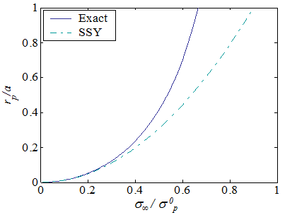
As the function $\sec(x)$ can be approximated by $\sec(x)= x +\frac{x^2}{2}+\frac{5x^4}{24}+\mathcal{O}(x^6)$, the small scale yielding assumption of Eq. (\ref{eq:cohesiveSize}) reads
\begin{equation} r_p=a\left(\sec\frac{\sigma_{\infty}{\pi}}{2\sigma_p^0}-1\right)\simeq \frac{a\pi^2}{8}{\left(\frac{\sigma_\infty}{\sigma_p^0}\right)}^2 \,.\label{eq:cohesiveSizeSSY}\end{equation}
The SSY approximation (\ref{eq:cohesiveSizeSSY}) is compared to the exact solution (\ref{eq:cohesiveSize}) in Picture VII.21, in which it can be seen that the SSY approximation remains accurate when the nominal loading $\sigma_\infty$ remains lower than $40\%$ of the yield stress $\sigma_p^0$.
The stress field of the yielding strip model
Using the process zone size (\ref{eq:cohesiveSize}), the stress distribution ahead of the cohesive zone is obtained from Eq. (\ref{eq:stressYieldStrip}). As the stress fields along the crack lips and along the process zone are known from the boundary conditions, the stress distribution for $y=0$ reads
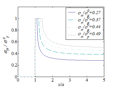
\begin{equation} \mathbf{\sigma}_{yy}\left(y=0\right) = \left\{\begin{array}{l } 0\text{ if } x<a\,;\\ \sigma_p^0 \text{ if } a<x<a+r_p\,;\\ \frac{2\sigma_p^0}{\pi}\text{arcotan}\left(\frac{a}{x}\sqrt{\frac{x^2-\left(a+r_p\right)^2}{r_p^2+2ar_p}}\right)\text{ if } a+r_p<x\,.\\ \end{array}\right.\label{eq:stressYieldStripFinal} \end{equation}
The stress distribution (\ref{eq:stressYieldStripFinal}) is illustrated in Picture VII.22 for different nominal loading values $\sigma_\infty$. It can be seen that the stress singularity is avoided with the yielding strip model.
The displacement field of the yielding strip model
Using the process zone size (\ref{eq:cohesiveSize}), the displacement field on the crack lips and on the process zone (\ref{eq:uYieldStrip}) is rewritten
\begin{equation} \mathbf{u}_y\left(\theta\rightarrow \pm \pi\right) = \pm \frac{\left(1+\nu\right)\left(1+\kappa\right) \sigma_p^0}{E\pi} \bigg[ a \text{arcoth} \sqrt{ \frac{\left(a+r_p\right)^2 - x^2}{r_p^2 + 2ar_p}} - x f\left(\frac{a}{x}\sqrt{ \frac{\left(a+r_p\right)^2 - x^2}{r_p^2 + 2ar_p}}\right) \bigg]\,, \label{eq:uYieldStripFinal}\end{equation}
where $f(f)$ is defined by Eq. (\ref{eq:ufCase3}). The Crack Opening Displacement (COD) $\delta$ is thus defined as
\begin{equation} \delta=[[ \mathbf{u}_y]] = 2\frac{\left(1+\nu\right)\left(1+\kappa\right)\sigma_p^0}{E\pi}\left[a \text{arcoth }\left(\sqrt{\frac{\left(a+r_p\right)^2-x^2}{r_p^2+2ar_p}}\right)-xf\left(\frac{a}{x}\sqrt{\frac{\left(a+r_p\right)^2-x^2}{r_p^2+2ar_p}}\right)\right]\,.\label{eq:CODYieldStrip} \end{equation}
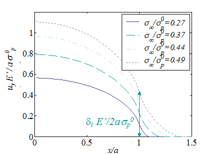
The displacement distribution (\ref{eq:uYieldStripFinal}) is illustrated in Picture VII.23 for different nominal loading values $\sigma_\infty$. It can be seen that at crack tip, i.e. for x=a, the opening is not zero. The Crack Tip Opening Displacement (CTOD) $\delta_t$ is therefore defined as the COD at $x=a$ and is derived as,
\begin{equation} \delta_t=\lim_{x\rightarrow{a^+}} [[\mathbf{u}_y]]\,,\label{eq:CTODDefinition} \end{equation}
where we have chosen arbitrarily the limit $x\rightarrow{a^+}$ from the upper side (both limits lead to the same result, but as the function $f(x)$ changes we need to choose one of them). From the COD field (\ref{eq:CODYieldStrip}), we thus have
\begin{equation} \delta_t = \lim_{x\rightarrow{a^+}} 8\frac{\sigma_p^0}{E'\pi}\left[a \text{arcoth} \left(\sqrt{\frac{\left(a+r_p\right)^2-x^2}{r_p^2+2ar_p}}\right) - x \text{arcoth} \left(\frac{a}{x} \sqrt{\frac{\left(a+r_p\right)^2-x^2}{r_p^2+2ar_p}}\right)\right]\,, \end{equation}
or using the identity $\text{arcoth} x = \frac{1}{2} \ln \frac{x+1}{x-1}$
\begin{equation} \begin{array}{rcl}\delta_t&=&\lim_{x\rightarrow{a^+}} 4\frac{\sigma_p^0}{E'\pi}\left[a \ln \left(\sqrt{\frac{\left(a+r_p\right)^2-x^2}{r_p^2+2ar_p}}+1\right) - a \ln \left(\sqrt{\frac{\left(a+r_p\right)^2-x^2}{r_p^2+2ar_p}}-1\right)\right. -\\&& \left.x \ln \left(\frac{a}{x}\sqrt{\frac{\left(a+r_p\right)^2-x^2}{r_p^2+2ar_p}}+1\right) +x \ln \left(\frac{a}{x} \sqrt{\frac{\left(a+r_p\right)^2-x^2}{r_p^2+2ar_p}}-1\right)\right]\,. \end{array}\end{equation}
As the limits of the first and third terms cancel each other, this equation becomes
\begin{equation} \delta_t = \lim_{x\rightarrow{a^+}} 4\frac{\sigma_p^0}{E'\pi}\left[- a \ln \left( \sqrt{\frac{\left(a+r_p\right)^2-x^2}{r_p^2+2ar_p}}-1\right) +x \ln \left(\frac{a}{x} \sqrt{\frac{\left(a+r_p\right)^2-x^2}{r_p^2+2ar_p}}-1\right)\right]\,, \end{equation}
which can be rewritten
\begin{equation} \delta_t=\lim_{x\rightarrow{a^+}} 4\frac{\sigma_p^0}{E'\pi} \left[a \ln \left( \frac{\frac{a}{x}\sqrt{\frac{\left(a+r_p\right)^2-x^2}{r_p^2+2ar_p}}-1}{\sqrt{\frac{\left(a+r_p\right)^2-x^2}{r_p^2+2ar_p}}-1}\right) + \left(x-a\right) \ln \left(\frac{a}{x}\sqrt{\frac{\left(a+r_p\right)^2-x^2}{r_p^2+2ar_p}}-1\right)\right]\,. \end{equation}
The limit of the second term tends to zero as a polynomial "wins" on a logarithm function, leading to
\begin{equation} \delta_t=\lim_{x\rightarrow{a^+}} 4\frac{\sigma_p^0 a}{E'\pi} \ln \left( \frac{\frac{a}{x}\sqrt{\frac{\left(a+r_p\right)^2-x^2}{r_p^2+2ar_p}}-1}{\sqrt{\frac{\left(a+r_p\right)^2-x^2}{r_p^2+2ar_p}}-1}\right)\,. \label{eq:CTODTmp}\end{equation}
The indetermination is removed by applying the Hospital's Theorem, yielding
\begin{equation}\begin{array}{lcl} \lim_{x\rightarrow{a^+}} \frac{\frac{a}{x}\sqrt{\frac{\left(a+r_p\right)^2-x^2}{r_p^2+2ar_p}}-1}{\sqrt{\frac{\left(a+r_p\right)^2-x^2}{r_p^2+2ar_p}}-1} &=& \lim_{x\rightarrow{a^+}} \frac{ -\frac{a}{x^2}\sqrt{\frac{\left(a+r_p\right)^2-x^2}{r_p^2+2ar_p}} - \frac{a}{\sqrt{r_p^2+2ar_p}\sqrt{\left(a+r_p\right)^2-x^2}}} {\frac{-x}{\sqrt{r_p^2+2ar_p}\sqrt{\left(a+r_p\right)^2-x^2}}} \\ &=& \lim_{x\rightarrow{a^+}}\frac{ -\frac{a}{x^2}\bigg(\left(a+r_p\right)^2-x^2\bigg)-a}{-x} = \frac{\left(a+r_p\right)^2}{a^2}\,,\end{array}\end{equation}
and Eq. (\ref{eq:CTODTmp}) becomes
\begin{equation} \delta_t=\lim_{x\rightarrow{a^+}} 8\frac{\sigma_p^0 a}{E'\pi} \ln \left(\frac{\left(a+r_p\right)}{a}\right)\,. \label{eq:CTODTmp2}\end{equation}
Using the size of the process zone (\ref{eq:cohesiveSize}), the CTOD $\delta_t$ is eventually rewritten as
\begin{equation} \delta_t=\lim_{x\rightarrow{a}}[[\mathbf{u}_y]]=8\frac{\sigma_p^0a}{E'\pi}\ln\left(\sec\frac{\sigma_\infty\pi}{2\sigma_p^0}\right)\,, \label{eq:CTODYieldStrip} \end{equation}
with
\begin{equation} E' = \frac{4E}{\left(1+\nu\right)\left(\kappa+1\right)} \left\{\begin{array}{ll} E &\text{ in plane-}\sigma\,;\\ \frac{E}{1-\nu^2}&\text{ in plane-}\varepsilon\,. \end{array} \right.\end{equation}
![]()