
Energetic Approach
This chapter introduces important concepts related to the energy released during a crack propagation. It is shown that the crack growth can be predicted based on energy principle, as predicted by Griffith formula $\sigma_{\text{TS}}\sqrt{a} \div \sqrt{E\, 2\gamma_s}$: the resistance of a structure could only be evaluated by considering its defects. The relation between the energy concept and the SIFs is also detailed. Particular emphasis is put on the applicability of the energetic methods and on the assumptions made.
Energetic Approach > Energy of cracked Bodies
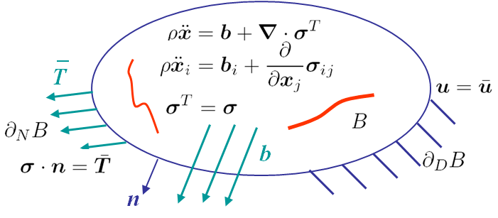
In this chapter we use the notations and governing equations previously detailed. The difference lies in the presence of cracks in the body B, as illustrated in Picture III.1. In this class we assume that these crack surfaces are stress-free.
As usually done to establish the principle of virtual work, let us consider a kinematically admissible field $\delta\mathbf{u}$ so that $\delta\mathbf{u}=0$ on $\partial_D B$, which multiplies the linear momentum balance equation. We can then integrate the resulting equation on the body and proceed with an integration by parts followed by the Gauss theorem, yielding
\begin{equation} \begin{cases} \int_B \mathbf{\nabla}\cdot\mathbf{\sigma}^T \cdot \delta\mathbf{u} dB + \int_B \mathbf{b}\cdot \delta\mathbf{u} dB = 0\\ \iff \int_B \mathbf{\sigma} : \delta\mathbf{\varepsilon} dB = \int_{\partial_N B} \bar{\mathbf{T}} \cdot \delta\mathbf{u} d\partial D + \int_B \mathbf{b}\cdot \delta\mathbf{u} dB\end{cases}\label{eq:pvw1} .\end{equation}
In the elastic regime (linear or not) the stress tensor derives from an internal potential $U$
\begin{equation} \mathbf{\sigma} = \partial_{\mathbf{\varepsilon}} U.\label{eq:Uint} \end{equation}
For example, in linear elasticity one has
\begin{equation} \mathbf{\sigma} = \mathcal{H}:\mathbf{\varepsilon} = \partial_{\mathbf{\varepsilon}} \frac{\mathbf{\varepsilon}:\mathcal{H}:\mathbf{\varepsilon}}{2} = \partial_{\mathbf{\varepsilon}} U.\label{eq:UintLinear} \end{equation}
Using (\ref{eq:Uint}) in the virtual work equation (\ref{eq:pvw1}) leads to
\begin{equation} \delta E_{\text{int}} = \delta \int_B U dB = \int_{\partial_N B} \bar{\mathbf{T}} \cdot \delta\mathbf{u} d\partial D + \int_B \mathbf{b}\cdot \delta\mathbf{u} dB = \delta W_{\text{ext}} \label{eq:pvw2},\end{equation}
which expresses the equality between the virtual work of the external forces and the virtual increment of internal energy. We can now analyze the energy changes when a crack propagates in a body $B$.
Body subjected to a prescribed loading (dead load)
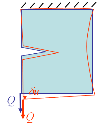
Let us assume that the body is under constant loading $\bar{\mathbf{T}}$ and $\mathbf{b}$. Assuming the crack surface is now different, the body deformation changes, and the body sees a displacement field $\delta \mathbf{u}$. Without loss of generalities we can represent this configuration by a general loading $Q$ at a loading point and a general displacement $\delta u$ at this loading point as shown in Picture III.2. Indeed, one has simply to define this general loading so that
\begin{equation} \begin{cases} \int_{\partial_N B} \bar{\mathbf{T}} d\partial D + \int_B \mathbf{b} dB = Q \left[ \int_{\partial_N B} \hat{\bar{\mathbf{T}}} d\partial D + \int_B \hat{\mathbf{b}} dB\right]\\ \delta \mathbf{u} = \delta u \hat{\mathbf{u}}\end{cases}\label{eq:genLoading},\end{equation}
where $ \hat{\bar{\mathbf{T}}} $ and $ \hat{\mathbf{b}}$ are unit loading corresponding to a displacement field $\delta \mathbf{u}$. From (\ref{eq:pvw2}) and (\ref{eq:genLoading}), assuming two different crack surfaces $A'$ and $A>A'$ for the same specimen under the constant loading $Q$, the loading point sees a displacement field $\delta u$, which corresponds to a work of the external forces
\begin{equation}\delta W_{\text{ext}} \int_{\partial_N B} \bar{\mathbf{T}} \cdot \delta\mathbf{u} d\partial D + \int_B \mathbf{b}\cdot \delta\mathbf{u} dB = Q\delta u \label{eq:wextPrescLoading}.\end{equation}
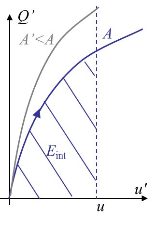
For the two crack surfaces, the internal energy of the body is also different. On the one hand the compliance and stiffness of the body $B$ is modified as the geometry changed, see Picture III.3, and on the other hand the body sees a displacement at the loading point. So the internal energy depends on the loading and on the crack surface
\begin{equation} E_\text{int} = E_\text{int}\left(Q,\, A\right). \label{eq:prescLoading1} \end{equation}
Finally $G$ is the energy associated to the creation of a (unit) crack surface. As $Q$ is constant, the balance of energy means that the work of external forces is used to change the internal energy and to create the surface, so that
\begin{equation} \delta E_\text{int} = Q\delta u - G \delta A = \delta\left(Qu\right) - G\delta A. \label{eq:prescLoading2}\end{equation}
From this equation we can define the energy release rate $G$ for a body under prescribed loading as
\begin{equation} G = - \partial_A \left( E_\text{int} - Q u\right). \label{eq:GPrescLoading} \end{equation}
This energy release rate is the energy released by the system (internal energy and work of external force) by unit increment of the crack surface.
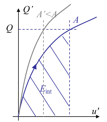
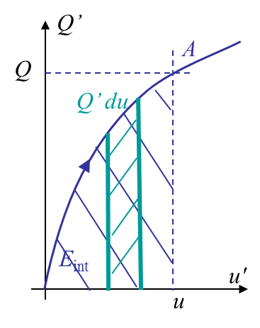
Let us now analyze the involved energies. Picture III.4 defines the complementary energy $u'\,dQ$ for a body of crack surface $A$. During the loading of the body -without crack propagation- the load $Q'$ ranges from 0 to $Q$ and the complementary energy reads
\begin{equation} Qu - E_\text{int} = \int_0^Q u\left(Q',\,A\right) dQ'.\label{eq:complementaryEnergyPrescLoading}\end{equation}
This equation allows the displacement field to be expressed for a given load $Q$ and for a given crack surface $A$ as
\begin{equation} u\left(Q,\,A\right) = - \partial_Q \left(E_\text{int}-Qu\right).\label{eq:uPrescLoading} \end{equation}
Comparing (\ref{eq:GPrescLoading}) and (\ref{eq:uPrescLoading}) allows writing
\begin{equation} \partial_Q G = \partial_A u \iff G = \int_0^Q \partial_A u\left(Q',\,A\right) dQ' . \label{eq:measuredGPrescLoading}\end{equation}
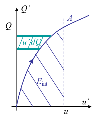
This equation gives the following physical meaning to $G$. Let us consider Picture III.5.
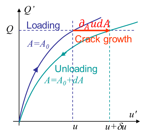
- A body of initial crack surface $A_0$ is loaded up to the point $Q'=Q$.
- Now the crack is assumed to propagate under constant loading to reach a surface $A_0 +dA$. As the compliance and stiffness of the body have changed the body sees an increase of the displacement from $u$ to $u+\delta u$.
- The body is then unloaded to reach $Q'=0$.
For the same value of $Q$, the difference in terms of displacement between the loading and unloading curves is easily obtained as $d u=\partial_A u\left(Q,\,A\right) dA$. Thus the surface between the two curves reads $\int_0^Q\partial_A u\left(Q',\,A\right) dQ'dA$. We now have the physical meaning of (\ref{eq:measuredGPrescLoading}) as the energy released rate multiplied by the surface increment $GdA$ is nothing else than the surface between two loading curves of a specimen with two different crack surfaces. This can be a way to measure $G$ either by finite-element or experimentally as one has just to load up to the same force a specimen with two different crack surfaces. This method has the advantage of not involving real crack propagation.
Note that in this section we do not know yet if the crack would propagate or not. We have analyzed the energy changes of a sample with two different crack sizes $A$ and $A+dA$ under prescribed loading.
Body subjected to a prescribed displacement
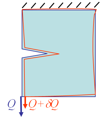
Let us now assume that the cracked body is subjected to a prescribed displacement $u$ at the loading point, see Picture III.6. For two different crack surfaces, as the displacement is constant, the reaction force is different as the compliance and stiffness of the sample are different due to the geometry change. The loading reaction changes from $Q$ to $Q+\delta Q$. Intuitively $\delta Q$ is negative as the compliance of the specimen increases with the crack surface.
Considering the same sample with two crack surfaces $A'$ and $A>A'$ under prescribed displacement. As the displacement is prescribed, the loading point does not move and does not induce a work:
\begin{equation}\delta W_{\text{ext}} = 0 \label{eq:wextPrescDisp}.\end{equation}
Nevertheless, the internal energy is different as the compliance and stiffness of the body are different, see Picture III.7. For the same displacement $u$ the loading reaction $Q$ is smaller for the larger crack surface, and so for the internal energy. So the internal energy depends on the displacement constraint and on the crack surface
\begin{equation} E_\text{int} = E_\text{int}\left(u,\, A\right). \label{eq:prescDisp1} \end{equation}
Finally $G$ is the energy associated to the creation of a (unit) crack surface. As $u$ is constant, the balance of energy means that the energy required to create the crack surface should come from the internal energy, so that
\begin{equation} \delta E_\text{int} = - G \delta A. \label{eq:prescDisp2}\end{equation}
From this equation we can define the energy release rate $G$ for a body under prescribed displacement as
\begin{equation} G = - \partial_A E_\text{int}. \label{eq:GPrescDisp} \end{equation}
This energy release rate is the energy released by the system from its internal energy by unit increment of the crack surface. Moreover, considering Picture III.8, which defines the internal energy increment $Q'dU$ for a body of crack surface $A$, leads to
\begin{equation} Q\left(u,\,A\right) = \partial_u E_\text{int}.\label{eq:QPrescDisp} \end{equation}
Comparing (\ref{eq:GPrescDisp}) and (\ref{eq:QPrescDisp}) allows writing
\begin{equation} -\partial_u G = \partial_A Q \iff G = - \int_0^u \partial_A Q\left(u',\,A\right) du' . \label{eq:measuredGPrescDisp}\end{equation}
This equation gives the following physical meaning to $G$. Let us consider Picture III.9.
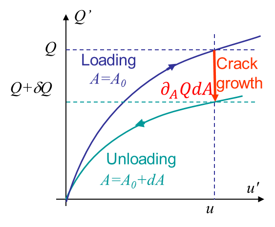
- A body of initial crack surface $A_0$ is loaded under displacement control up to the point $u'=u$.
- Now the crack is assumed to propagate under constant constrained displacement to reach a surface $A_0 +dA$. As the compliance and stiffness of the body have changed the body sees a decrease of the reaction force from $Q$ to $Q+\delta Q<Q$.
- The constrained displacement is then relaxed to reach $u'=0$.
For the same value of $u$, the difference in terms of reaction force between the loading and unloading curves is easily obtained as $d Q=\partial_A Q\left(u,\,A\right) dA$ (<0). Thus the surface (>0) between the two curves reads $-\int_0^u\partial_A Q\left(u',\,A\right) du'dA$. We now have the physical meaning of (\ref{eq:measuredGPrescDisp}) as the energy released rate multiplied by the surface increment $GdA$ is nothing else than the surface between two loading curves of a specimen with two different crack surfaces. As for the prescribed force loading case, this can be used to measure $G$ without involving crack propagation.
Note that in this section we do not know yet if the crack would propagate or not. We have analyzed the energy changes of a sample with two different crack sizes $A$ and $A+dA$ under prescribed loading.