
Crack Growth > Fatigue Failure
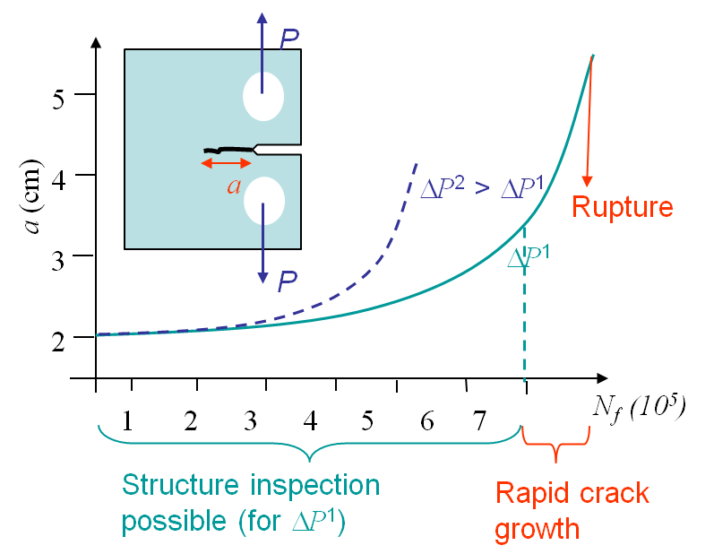
While subjected to a cyclic loading, see Picture V.28, a structure can be softened due to the apparition and the propagation of a crack, that can be initiated and propagated for loadings such that $\sigma < \sigma_p^0$ and $K_I < K_{IC}$. Let us consider a specimen under cyclic loading as described on Picture I.71. The value of $P$ ranges from $P_\text{min}$ to $P_\text{max}$ so that $\Delta P = P_\text{max} - P_\text{min}$. Due to the cyclic loading a crack nucleates at the stress concentration and propagates until failure of the specimen, although at the beginning the SIF remains lower than $K_{IC}$, see Picture V.28.
Phenomenological explanations
Microscopic observations of structures which failed by fatigue show:
- Cracks are initiated at stress concentration points;
- Micro-scopic crack growth along the crystal slip planes (Stage I);
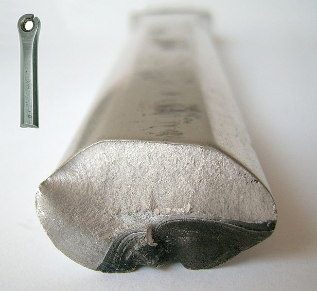
- Macro-scopic crack growth with surface striations, see Picture V.29 Dark zone (Stage II);
- Failure of the structure occurs when the crack reaches a critical size, see Picture V.29 Bright zone (Stage III).
The phenomenological explanations of these stages was reported in the overview.
Prediction of the structural life
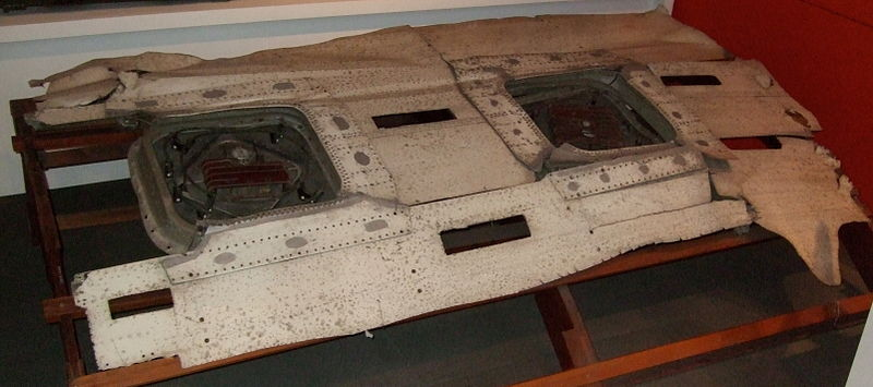
As discussed in the overview, with the example of the Comet, see Picture V.30, a safe life approach is unable to predict the life of a structure under cyclic loading when some defects initially exist. A new theory was developed for the purpose of predicting the crack growth and the end of life of a given structure subjected to a cyclic loading. This theory, known as the damage tolerant design, assumes that defects exist in the structure at the end of their manufacturing (or from the start of their service), or because of accidents.
The question is now how can we predict the evolution of the crack size, and the failure point, in terms of the cycles number. In other words, how can we predict the curves of Picture V.28.
As the crack loading remains small during fatigue problems, the SSY assumption usually holds during some intervals of the crack growth or even until failure, depending on the case. As at the macro-scale the life of the structure with an initial crack size $a$ is observed to depend on the loading $\Delta P$ and on $\frac{P_\text{max}}{P_\text{min}}$ only, the SSY assumption allows us to say that the conditioning parameters are $\Delta K$ and $R = \frac{K_\text{max}}{K_\text{min}}$. Indeed from the SIFs equations we observed a linearity in $\Delta P$ of $\Delta K$. Therefore the evolution of the crack size obeys to
\begin{equation} \frac{d a}{d N_f} = f\left(\Delta K, R\right). \label{eq:dadN}\end{equation}
With the knowledge of this curve it is possible to determine for the number of cycles a structure can sustain before being replaced and to schedule the inspection intervals. Note that the uncertainty on this curve can reach several (tens of) percent, so regular intervals are thus required to validate or modify the prediction.
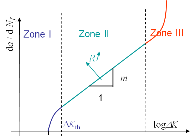
What remains to be defined now is the form of $f\left(\Delta K, R\right)$ in (\ref{eq:dadN}). Experimentally it has been found that this function follows the curve shown in Picture V.31.
Crack propagation in Stage I
Experimentally, it has been observed that if $\Delta K < \Delta K_\text{th}$, where $\Delta K_\text{th}$ the crack growth is in average smaller than one atomic spacing per cycle. Such a crack is considered as dormant. The value of $\Delta K_\text{th}$ is the fatigue threshold and depends on the material but also on the loading ratio $R$.
If $\Delta K > \Delta K_\text{th}$, the crack will propagate until reaching the stage II.
For steel, $\Delta K_\text{th}$ is between 2 and 5 $\text{MPa}\cdot\sqrt{\text{m}}$, but for steel in sea water, $\Delta K_\text{th}$ is between 1 and 1.5 $\text{MPa}\cdot\sqrt{\text{m}}$. This means that the environmental conditions in which the material is considered are very important.
Crack propagation in Stage II
\begin{equation} \frac{d a}{d N_f} = C \Delta K ^m.\label{eq:Paris} \end{equation}
This law is characterized by two parameters $C$ and $m$ which depend on the material and on the loading ratio $R$. For steel, $C \approx 0.1\times 10^{-11}$ $\text{m}\cdot\left(\text{MPa}\cdot\sqrt{\text{m}}\right)^{-m}$ and $m \approx$ 4. For steel in sea water, these values change a lot: $C \approx 1.6 \times 10^{-11}$ $\text{m}\cdot\left(\text{MPa}\cdot\sqrt{\text{m}}\right)^{-m}$ and $m \approx$ 3.3. This means that the environmental conditions in which the material is considered are very important. Note that the units of $C$ are cumbersome as they depend on the coefficient $m$.
When applying the Paris law, it is important to remember that $K$ depends on the crack size. Thus $\Delta K$ should be replaced by its complete expression when integrating to get $a(N_f)$. For instance, for Mode I in an infinite plate, we have:
\begin{equation} K_I = \sigma_\infty \sqrt{\pi a}, \end{equation}
and $\Delta K$ is given by:
\begin{equation} \Delta K = \left(\sigma_{\infty,\text{max}}-\sigma_{\infty,\text{min}}\right) \sqrt{\pi a}. \end{equation}
Crack propagation in Stage III
In this zone the crack grows rapidly until failure of the structure. The failure is reached as soon as the crack size reaches $a_f$ such that $K(P_\text{max},\,a_f)$ is equal to $K_c$.
Typical material parameters
| Material | $\Delta K_{\text{th}} \text{ [MPa }\cdot\sqrt{\text{m}}\text{]}$ | $m$ [-] | $C \text{ [}m\left(\text{MPa }\cdot\sqrt{\text{m}}\right)^{-m}\text{]}$ |
|---|---|---|---|
| Mild steel |
3.2-6.6 |
3.3 | $0.24 \cdot 10^{-11}$ |
| Structural steel |
2.0-5.0 |
3.85-4.2 | $0.07-0.11 \cdot 10^{-11}$ |
| Structural steel is sea water |
1.0-1.5 |
3.3 | $1.6 \cdot 10^{-11}$ |
| Aluminum | 1.0-2.0 | 2.9 | $4.56 \cdot 10^{-11}$ |
| Aluminum alloy |
1.0-2.0 | 2.6-2.9 | $3-19 \cdot 10^{-11}$ |
| Copper |
1.8-2.8 | 3.9 | $0.34 \cdot 10^{-11}$ |
| Titanium alloy (6Al-4V, R=0.1) |
2.0-3.0 | 3.22 | $1 \cdot 10^{-11}$ |
Effects of $R$: Crack closure
As explained, the loading ratio $R$ has an effect on the fatigue crack propagation. During the loading phases at maximum stress,
- There is an active plastic zone (phase transformation can happen);
- The crack opening allows fluid or products to enter.
Because of these effects, i f $R$ is low (< 0.7) or negative the crack lips can enter into contact at low stress values due to:
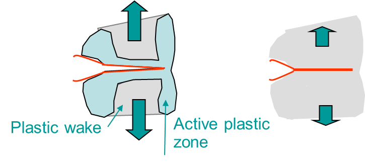
- Plasticity: the residual plastic strain resulting from the plastic wake closes the crack, see Picture V.32;
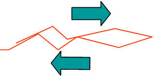
- Roughness: the roughness of the crack lips prevents sliding in Mode II, see Picture V.33;

- Corrosion: the corrosion products fill the crack and prevent it to close, see Picture V.34;

- Viscous fluid: lubricant fluids fill the crack and prevent it to close, see Picture V.35;

- Phase transformation: the change of volume at crack tip puts the material into compression, see Picture V.36.
Effect of the crack closure on fatigue
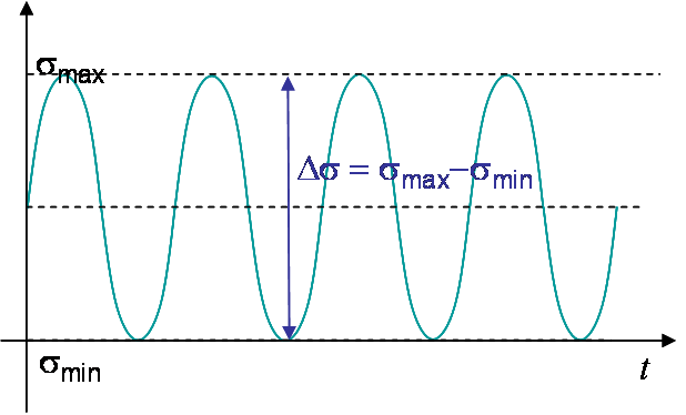
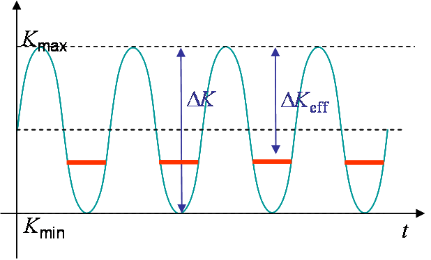
Because of the crack closure effect described here above, when the loading decreases, local compressive effects appear and parts of the cracks are kept opened. The SIFs at the minimum of the cycles defined in Picture V.37, are higher than expected as shown in Picture V.38. Hence the effective $\Delta K$ is actually reduced and the crack closure effect is therefore beneficial to the structure life.
Effect of $R$ on the threshold in zone I
Due to the Plasticity Induced Crack Closure (PICC), $\Delta K_\text{th}$ decreases when $R$ increases. Low values of $R$ are thus beneficial on the crack initiation. The ratio in the threshold can reach values of 5.
Effect of $R$ on the crack growth rate
Due to the crack closure, the life of the structure is improved for low $R$, as depicted in Picture V.31. Example for 2024-T3 aluminum alloy can be found in "J.C. Newman Jr, E.P. Phillips, M.H. Swain, Fatigue-life prediction methodology using small-crack theory, International Journal of Fatigue 21, 1999".
In order to unify the Paris law for different loading ratios $R$, models exist to evaluate the effective SIF $\Delta K_\text{eff}$. For example, the model of Elber & Schijve for Al. 2024-T3 suggests that $\Delta K_\text{eff} = (0.55 + 0.33 R + 0.12 R^2)\Delta K$ for $-1 < R < 0.54$. The use of such models is really delicate: models can be inaccurate in non-adequate circumstances (loading, environment, ), and are material dependent!
Overload effect
During a structure operation, the loading is never as regular as depicted in Picture V.37. What happens if there is a few (or a moderate) number of overloads?
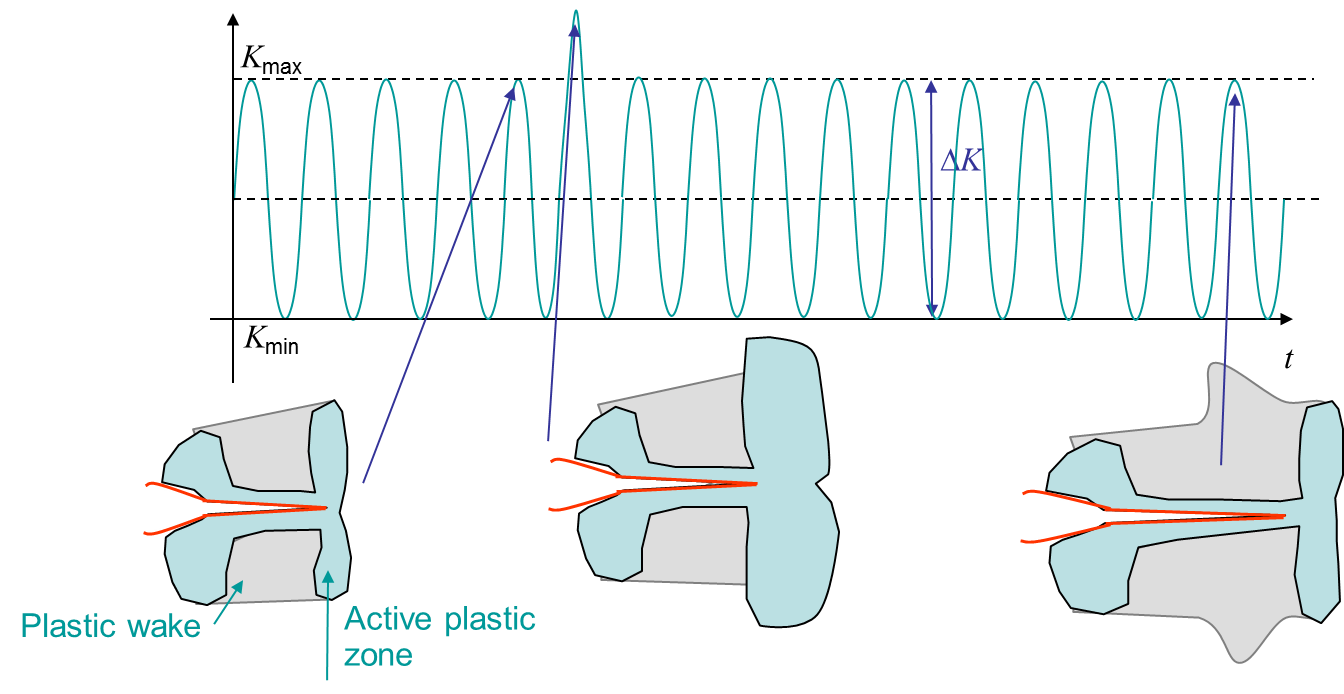
Let us consider the cyclic loading with an overload as illustrated in Picture V.39:
- Before the overload, the crack propagates with its plastic wake;
- During the overloading, the active plastic zone is higher than for the other cycles;
- The plastic wake is temporarily increased (Phase 1) for the coming cycles until the active plastic zone at the crack tip passes the plastic zone created by the overload (Phase 2);
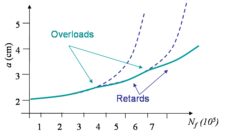
- During Phase 1, $\Delta K_\text{eff}$ is reduced due to the PICC and the crack propagates slower: there exists a retard effect in the crack propagation rate as illustrated in Picture V.40.
- Once the crack tip has passed the modified wake in Phase 2, $\Delta K_\text{eff}$ is as expected and the initial propagation rate is recovered as illustrated in Picture V.40.
- However, too frequent overloads are damaging as they actually correspond to increasing $K_\text{max}$.
Note that in 1952, the De Havilland Comet I fuselage was tested against fatigue following this scheme:
- Static loading at 1.12 atm;
- 10 000 cycles at 0.7 atm (larger than the cabin pressurization of 0.58 atm);
but the production fuselages without the first static loading failed after a few thousand cycles at 0.58 atm. The reason is that the production fuselages did not beneficiate from the PICC of the tested fuselage induced by the static loading.
The last reason for crack to propagate is due to corrosion.
![]()