
Cohesive Zone > Insights of Dugdale's model
Dugdales experiments
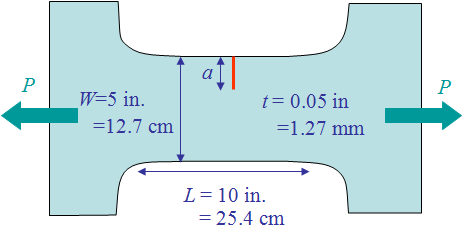
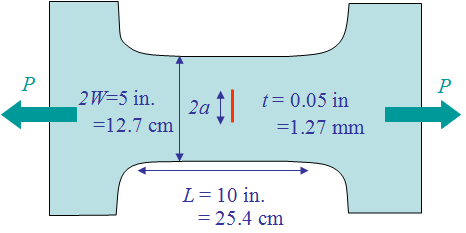
Dugdale has conducted experiments using a mild steel specimen (0.05% C, 0.4% Mn, 0.013% N), that was annealed at 900°C after being cut. The Yield strength of the material is ${\sigma_p}^0$ = 190 MPa and the Young's modulus is $E$ = 210 GPa. Dugdale has considered two different cases: one consisting of specimens with an edge crack as shown in Picture VII.24; and one consisting of specimens with a centered crack as shown in Picture VII.25. Several initial crack lengths $a$ were considered, but they remained small compared to the width $W$ of the specimen ($\leq 10 \%$). Several values of the load were tested on the specimen as to approach to yielding, however care was taken of not to propagate the crack (these are not fracture tests). The load was then released and the specimens cut, polished, and etched so that to measure the size of the process zone $r_p$ resulting from the loading test. The different crack lengths and loading conditions are reported in Table VII.1 along with the measurements of the process zone $r_p$.
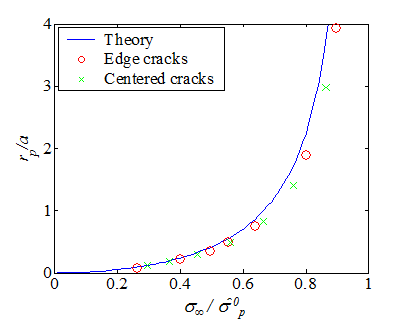
The results from the experiments are reported in Picture VII.25 where they are compared to the theoretical values of the process zone $r_p$. Results from the experiments for the two different cases compare very well to each other and also to the theoretical values of the process zone $r_p$. Note that the model holds for centered crack and edge cracks as long as the assumption $ a+r_p << W $ (infinite plate assumption) holds.
Relation with the J-integral
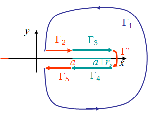
Assuming there is no unloading of the specimen, i.e. no crack propagation, an internal potential $U\left(\mathbf{\varepsilon}\right)$ can be defined for perfectly plastic J2-material. Therefore, the J-integral can be evaluated. The J-integral is path independent and the J-integral on a contour $\Gamma_1$ that embeds the crack tip and the process zone can be evaluated by selecting a contour that surrounds closely the process zone as illustrated on Picture VII.27, with
\begin{equation} \begin{array}{lcl} J &=& \int_{\Gamma_1}\left[U\left(\mathbf{\varepsilon}\right)\mathbf{n}_x-\mathbf{u}_{,x}\cdot\mathbf{\sigma}\cdot\mathbf{n}\right]dl\\ &=& - \int_{\Gamma_2+\Gamma_3+\Gamma'+\Gamma_4+\Gamma_5}\left[U\left(\mathbf{\varepsilon}\right)\mathbf{n}_x-\mathbf{u}_{,x}\cdot\mathbf{\sigma}\cdot\mathbf{n}\right]dl\end{array} \label{eq:JCohesiveZone1}\,,\end{equation}
where, $\Gamma$, $\Gamma_1$, $\Gamma_2$, $\Gamma_3$, $\Gamma_4$, and $\Gamma_5$ define the contour surrounding closely the process zone. The J-integral is thus computed as follows:
- On contour parts $\Gamma_2$ and $\Gamma_5$: $\mathbf{n}_x=0$ and the crack is free from stresses so their contribution to J-integral is zero;
- On contour parts $\Gamma'$: As the length of $\Gamma'$ tends toward zero when the contour gets closer from the process zone, its contribution to the J-integral vanishes;
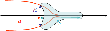
- On the contour part $\Gamma_3$ (respectively $\Gamma_4$): $\mathbf{n}_x=0$, but $\mathbf{\sigma}\cdot\mathbf{n} = - \sigma_y(\delta) \mathbf{e}_y (+ \sigma_y(\delta) \mathbf{e}_y)$ and $dl = dx (-dx)$, where $\sigma(\delta)$ represents the evolution of the stress on the process zone with the COD $\delta$, see Picture VII.7 for Dugdale's model and Picture VII.11 for Barenblatt's model.
Using these results allows rewriting Eq. (\ref{eq:JCohesiveZone1}) as
\begin{equation} J=-\int_{\Gamma_3}\mathbf{u}_{y,x}\mathbf{\sigma}_y\left(\delta\right)dx - \int_{\Gamma_4}\mathbf{u}_{y,x}\mathbf{\sigma}_y\left(\delta\right)dx = - \int_a^{a+r_p}\left[[u_y\right]]_{,x} \mathbf{\sigma}_y\left(\delta\right)dx \,,\label{eq:CohesiveZone2}\end{equation}
or again, as the COD $\delta$ is defined by $\delta = \left[[u_y\right]]$, as
\begin{equation} J = - \int_a^{a+r_p}\delta_{,x}\mathbf{\sigma}_y\left(\delta\right)dx= - \int_{\delta_t}^0 \mathbf{\sigma}_y \left(\delta\right)d\delta = \int_0^{\delta_t} \mathbf{\sigma}_y\left(\delta\right)d\delta \label{eq:JCohesiveZone}\,.\end{equation}
This result, which is valid for both Barenblatt's and Dugdale's models, shows that the flow of energy toward the process zone corresponds to the separation energy of the cohesive zone. Therefore the J-integral can be used in plasticity and could be used as a crack growth criterion, i.e. the crack would grow if $J=J_C$. This criterion could also be rewritten in terms of a critical crack tip opening $\delta_t = \delta_C$.
For the particular case of Dugdale's model, $\sigma(\delta)$ is constant for $\delta\leq\delta_t$ and is equal to $\sigma_p^0$ see Picture VII.7. Therefore, the J-integral (\ref{eq:JCohesiveZone}) is rewritten as,
\begin{equation} J_\text{Dugdale} = \mathbf{\sigma}_p^0 \int_0^{\delta_t} d\delta = \mathbf{\sigma}_p^0\delta_t \,.\label{eq:JDugdale}\end{equation}
In this case, a criterion on $J$ is directly related to a maximal value of $\delta_t$ as $J_C = \delta_{C}$ ${\sigma_p}^0$.
Finally, in the case of a plate large enough compared to the crack size, using the value of the Crack Tip Opening Displacement (CTOD), Eq. (\ref{eq:JDugdale}) leads to
\begin{equation} J_\text{Dugdale} = \mathbf{\sigma}_p^0\delta_t = 8 \frac{\left(\sigma_p^0\right)^2a}{E'\pi}\ln\left(\sec\frac{{\sigma}_\infty\pi}{2{\sigma}_p^0}\right)\,.\label{eq:JDugdaleInf}\end{equation}
Extension of LEFM to elastic-perfectly plastic materials
We have seen that for elastic-perfectly plastic materials, a criterion for crack growth is $J >= J_C$. However in some cases it is possible to extend the LEFM theory to elastic-perfectly plastic materials if there is no extensive plasticity prior to fracture, that is if the plastic zone remains small compared to characteristic lengths. In that case, the SIF $K$ could still be used as a crack growth criterion by defining the concept of an effective crack length.
Effective crack length
The idea behind this concept is to add a part $\eta$ of the process zone $r_p$ to the crack size $a$ in order to define the effective crack length
\begin{equation} a_\text{eff} = a + \eta r_p \,,\label{eq:aeff}\end{equation}
from which the SIF is evaluated as $K\left(a_\text{eff}\right)$. The factor $\eta$ is determined so that the $J$ value computed from the SIF corresponds to the J-integral, i.e.
\begin{equation} J = \frac{K_I^2\left(a_\text{eff}\right)}{E'} \label{eq:JSIF}\,. \end{equation}
For the case of Mode I loading of an infinite plane, one has $K_I = {\sigma}_\infty\sqrt{\pi a_{eff}}$, and using Eq. (\ref{eq:JDugdaleInf}), Eq. (\ref{eq:JSIF}) becomes
\begin{equation} J = 8\frac{\left({\sigma}_p^0\right)^2a}{E'\pi}\ln\left(\sec\frac{{\sigma}_\infty\pi}{2{\sigma}_p^0}\right) = \frac{K_I^2\left(a_\text{eff}\right)}{E'} = \frac{\pi{\sigma}_\infty^2 a_\text{eff}}{E'}\,. \label{eq:JSIFInf}\end{equation}
So the effective length is found to be
\begin{equation} a_\text{eff} = \frac{8a}{\pi^2} {\left(\frac{{\sigma}_p^0}{{\sigma}_\infty}\right)}^2 \ln \left(\sec\frac{{\sigma}_\infty\pi}{2{\sigma}_p^0}\right)\,.\label{eq:aEffInf}\end{equation}
If $\sigma_\infty < {\sigma_p}^0$, as the function $\sec(x)$ can be approximated by $\sec(x)= x +\frac{x^2}{2}+\frac{5x^4}{24}+\mathcal{O}(x^6)$ and the function $\ln(1+x)$ by $\ln(1+x)= x - \frac{x^2}{2}+\mathcal{O}(x^3)$, the small scale yielding (SSY) assumption of the effective length reads
\begin{equation}\begin{array}{lcl} a_\text{eff} &\simeq& \frac{8a}{\pi^2} {\left(\frac{{\sigma}_p^0}{{\sigma}_\infty}\right)}^2 \ln \left(1+\frac{1}{2}{\left(\frac{{\sigma}_\infty\pi}{2{\sigma}_p^0}\right)}^2+ \frac{5}{24}{\left(\frac{{\sigma}_\infty\pi}{2{\sigma}_p^0}\right)}^4\right)\\ &\simeq & \frac{8a}{\pi^2} {\left(\frac{{\sigma}_p^0}{{\sigma}_\infty}\right)}^2 \left(\frac{1}{2}{\left(\frac{{\sigma}_\infty\pi}{2{\sigma}_p^0}\right)}^2+\frac{5}{24}{\left(\frac{{\sigma}_\infty\pi}{2{\sigma}_p^0}\right)}^4-\frac{1}{8}{\left(\frac{{\sigma}_\infty\pi}{2{\sigma}_p^0}\right)}^4\right)\,. \end{array} \label{eq:aEffSSY}\end{equation}
This equation allows $\eta$ to be identified since the size of the process zone under SSY assumption is $r_p\simeq\frac{a\pi^2}{8}{\left(\frac{\sigma_\infty}{\sigma_p^0}\right)}^2$. One has thus
\begin{equation} a_\text{eff} = a + \eta{r_p} \simeq a + \frac{a}{24} {\left(\frac{{\sigma}_\infty\pi}{{\sigma}_p^0}\right)}^2 = a + \frac{r_p}{3}\,, \label{eq:aEffEta}\end{equation}
and, for SSY, one has $\eta$ = $\frac{1}{3}$.
Finally, by combining Eq. (\ref{eq:JSIFInf}), Eq. (\ref{eq:aEffInf}) and Eq. (\ref{eq:aEffEta}), the CTOD $\delta_t$ can be computed from $a_\text{eff}$ as $J = {\sigma}_p^0\delta_t = \frac{\pi{{\sigma}_\infty^2}a_\text{eff}}{E'}$ and an SSY approximation can be obtained
\begin{equation} \delta_t = \frac{\pi{\sigma}_\infty^2 a_\text{eff}}{E' {\sigma}_p^0} \simeq \frac{\pi {\sigma}_\infty^2 a}{E' {\sigma}_p^0}+\frac{\pi^3{\sigma}_\infty^4 a}{24E' \left(\sigma_p^0\right)^3}\,.\label{eq:CTODSSY} \end{equation}
Validity of Small Scale Yielding (SSY) Assumption
In order to assess the accuracy of the SSY assumption, the sizes of the process zone $r_p$ and the values of the J-integral, obtained using the Dugdale's model and its SSY approximation for a crack size $a$ small compared to the plate width $W$ under Mode I loading condition, are compared to each other.
First, the sizes of the process zone using Dudgale's model and under SSY assumption read
\begin{equation} r_p=a\left(\sec\frac{\sigma_{\infty}{\pi}}{2\sigma_p^0}-1\right)\simeq \frac{a\pi^2}{8}{\left(\frac{\sigma_\infty}{\sigma_p^0}\right)}^2 \,.\label{eq:cohesiveSizeSSY}\end{equation}
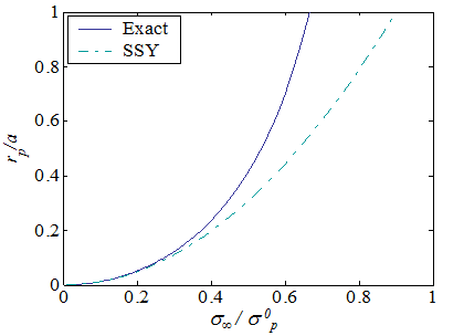
The SSY approximation (\ref{eq:cohesiveSizeSSY}) is compared to the exact solution in Picture VII.21, in which it can be seen that the SSY approximation remains accurate when the nominal loading $\sigma_\infty$ remains lower than $40\%$ of the yield stress $\sigma_p^0$. In that case, the extension of the process zone $r_p$ remains lower than 20$\%$ of the crack size $a$.
In order to extract the SSY approximation of the J-integral, we consider the exact value of $a_\text{eff}$ (\ref{eq:aEffInf}), and its SSY approximation (\ref{eq:aEffEta}) leading to,
\begin{equation} a_\text{eff} = \frac{8a}{\pi^2}{\left(\frac{{\sigma}_p^0}{{\sigma}_\infty}\right)}^2 \ln \left(\sec\frac{{\sigma}_\infty\pi}{2{\sigma}_p^0}\right) \simeq a+\frac{a}{24}{\left(\frac{{\sigma}_\infty\pi}{{\sigma}_p^0}\right)}^2\,.\label{eq:aEffSSYbis} \end{equation}
Hence the SSY approximation of the J-integral (\ref{eq:JSIFInf}) turns out to be
\begin{equation} \begin{array}{lll} J = \frac{\pi{{\sigma}_\infty^2}a_\text{eff}}{E'} &=& \frac{8a{\left({\sigma}_p^0\right)}^2}{\pi{E'}}\ln\left(\sec\frac{{\sigma}_\infty\pi}{2{\sigma}_p^0}\right)\\ &\simeq&\frac{\pi{\sigma}_\infty^2a}{E'}+\frac{\pi{\sigma}_\infty^2a}{24E'}{\left(\frac{{\sigma}_\infty\pi}{{\sigma}_p^0}\right)}^2 \end{array}\,.\label{eq:JSSY}\end{equation}
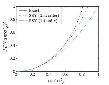
The SSY approximation of the J-Integral consists of a first order term in $\sigma_\infty^2$ and of a second order term in $\sigma_\infty^2\left(\frac{\sigma_\infty}{\sigma_p^0}\right)^2$ as seen in Eq. (\ref{eq:JSSY}). The different approximations and the exact J-integral values are illustrated in Picture VII.29. It can thus be concluded that, if $\sigma_{\infty}< 40\%$ of $ {\sigma_p}^0$, then a first order SSY (or simply LEFM) assumption holds, while for $\sigma_{\infty}< 60\%$ of $ {\sigma_p}^0$, the LEFM and SSY assumptions can still be considered, but only if $a_\text{eff}$ is used. Note that for $\sigma_{\infty}< 60\%$ of $ {\sigma_p}^0$, the process zone length $r_p$ extend up to 70$\%$ of the crack length $a$, see Picture VII.28, so that the criterion $a \geq 1.4 r_p$ can be used to assess this case.
First order SSY (LEFM) assumption for Dugdales model
As seen earlier for an infinite plate in Mode I loading, if $\sigma_{\infty}< 40\%$ of $ {\sigma_p}^0$, then a first order SSY (i.e. LEFM theory) assumption holds. LEFM can still be applied because the process zone has a size limited to $r_p < 20\%$ of $a$, see Picture VII.28. For an infinite plate in mode I, the J-integral reduces to $J = \frac{\pi{\sigma}_\infty^2 a}{E'} = \frac{K_I^2\left(a\right)}{E'}$. The concept of LEFM holds without any correction of the crack size and, using Eq. (\ref{eq:aEffEta}) and as $K_I=\pi \sigma_\infty\sqrt{a}$, the size of the plastic zone (process zone) is $r_p \simeq \frac{\pi}{8}{\left(\frac{K_I}{{\sigma}_p^0}\right)}^2$.
Other geometries and loading conditions can also be considered as the results were shown to hold by considering finite element simulations e.g., in which case one has still $J = \frac{K_I^2\left(a\right)}{E'}+\frac{K_{II}^2\left(a\right)}{E'}+\frac{K_{III}^2\left(a\right)}{2\mu}$ and under mode I loading $r_p \simeq \frac{\pi}{8}{\left(\frac{K_I}{{\sigma}_p^0}\right)}^2$.
Therefore, a criterion to assess whether LEFM can be applied is to make sure that the plastic zone computed using the first order SSY assumption $r_p$ remains lower than $ 20\%$ of $a$. This LEFM criterion thus reads
\begin{equation} a,\,L ≥ \frac{5\pi}{8} {\left(\frac{K_I}{{\sigma}_p^0}\right)}^2 \simeq 2{\left(\frac{K_I}{{\sigma}_p^0}\right)}^2\,,\label{eq:DugdaleLEFMCriterion}\end{equation}
where $L$ corresponds to other characteristic sizes such as the ligament. In the case the crack growth is assessed, $K_C$ should be used instead of $K_I$ in Eq. (\ref{eq:DugdaleLEFMCriterion}).
Another finding of Dugdale's model it that the CTOD, i.e. the opening at crack tip, is not zero. Therefore there is a blunting of the crack tip due to the cohesive zone
\begin{equation} \delta_t = \frac{J}{{\sigma}_p^0} = \frac{K_I^2}{E'{\sigma}_p^0}\,.\label{eq:CTODfromJ} \end{equation}
A fracture criterion based on the CTOD can therefore also be considered. Such a criterion reads $\delta_t = \delta_C = \frac{K_C^2}{E'{\sigma}_p^0}$ with the critical opening $\delta_C$ that can be measured experimentally.
These relations are valid for Dugdales model only, that is, for thin sheets (plane stress: $r_p >> t$) in which case $E = E$; for Low-C steel (perfectly plastic); and for Glassy polymers as discussed earlier.
Second order SSY (LEFM with Effective Crack Length) assumption for Dugdales model
If $40\%{\sigma_p}^0<\sigma_{\infty}< 60\%{\sigma_p}^0$, then a second order SSY assumption can be used. For an infinite plate under Mode I loading, the process zone $r_p $ extends and can reach up to 70% of the crack size $a$, see Picture VII.28. The J-integral can still be computed from the SIF, but only by considering the effective crack length: $J = \frac{K_I^2\left(a_\text{eff}\right)}{E'}$ with $K_I={\sigma}_\infty\sqrt{\pi a_{eff}}$, see Picture VII.29. The effective crack length is computed from Eq. (\ref{eq:aEffSSYbis}), and for an infinite plate under Mode I loading one has
\begin{equation} a_\text{eff} = a+\frac{r_p}{3}\text{ with }\frac{r_p}{3} \simeq \frac{a_\text{eff}}{24}{\left(\frac{{\sigma}_\infty\pi}{{\sigma}_p^0}\right)}^2 \simeq \frac{\pi}{24} {\left(\frac{K_I\left(a_\text{eff}\right)}{{\sigma}_p^0}\right)}^2\,.\label{eq:EffectiveCrackSSYInf} \end{equation}Other geometries and loading conditions can also be considered as the results were shown to hold by considering finite element simulations e.g., in which case one has still $J = \frac{K_I^2\left(a_\text{eff}\right)}{E'}+\frac{K_{II}^2\left(a_\text{eff}\right)}{E'}+\frac{K_{III}^2\left(a_\text{eff}\right)}{2\mu}$ and under Mode I loading $r_p \simeq \frac{\pi}{8}{\left(\frac{K_I(a_\text{eff})}{{\sigma}_p^0}\right)}^2$. Note that when evaluating the size of the cohesive zone, one should use $K(a_\text{eff})$ as
\begin{equation} a_\text{eff} = a+\frac{r_p}{3}\text{ with }\frac{r_p}{3} \simeq \frac{\pi}{24} {\left(\frac{K_I\left(a_\text{eff}\right)}{{\sigma}_p^0}\right)}^2\,,\label{eq:EffectiveCrackSSY} \end{equation}
and not $K(a)$ which is only first order accurate. There is therefore an iterative procedure to follow as shown below:
- Step 1: Compute $K$ from $a$;
- Step 2: Compute effective crack size $a_\text{eff}$ from Eq. (\ref{eq:EffectiveCrackSSY});
- Step 3: Compute an updated value for $K$ from $a_\text{eff}$ and go back to step 2, if needed.
As mentioned earlier, these relations are valid for Dugdales model only, that is, for thin sheet (plane stress: $r_p >> t$) in which case $E = E$; for Low-C steel (perfectly plastic); and for Glassy polymers.
Summary of Dugdales model insights
According to the previous analysis, the SSY assumption can be used under some circumstances:
- If ${\sigma}_\infty < 40\% $ of ${\sigma}_p^0$ and $a,\,L > 5 r_p $, then first order SSY can be used, where $L$ referred to characteristic sizes such as the ligament. Therefore, the classical LEFM solutions can be used.
- If ${\sigma}_\infty < 60\% $ of ${\sigma}_p^0$ and $a,\,L> 1.4 r _p $, then second order SSY should be used. Therefore, the classical LEFM solutions can be used provided the crack size is corrected to obtain an effective crack size which consists of an iterative procedure to follow.
- If ${\sigma}_\infty > 60\% $ of ${\sigma}_p^0$, then the J integral should be computed (in this chapter we have only considered the J-integral of an infinite plane, but we have seen how to compute it in the general case. The crack growth criterion should thus be based on this J-integral, i.e. $J\geq J_C = \delta_C\sigma_p^0$. Also, the remaining ligament $L$ should be greater than $r_p$ for the theory of the J-integral to hold as it will be seen in the next Chapter.
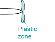
Note that these relations are valid for Dugdales model only, that is, for thin sheest; Low-C steel (perfectly plastic materials); and for Glassy polymers. For elasto-plastic materials in plane strain conditions, the plastic zone has a different shape see Picture VII.31 and another model should be developed, which is the purpose of the next chapter.