
Overview > Linear Elastic Fracture Mechanics (LEFM)
Why do we need fracture mechanics?
You might be wondering why is it necessary to develop a whole theory taking into account a microscopic defect (the crack) to describe the behavior at the macroscopic scale. There are two reasons for this:
- It is impossible to produce a crack free structure and we have seen that accounting for the existing defects is required to predict the life of the structure.
- If we apply classical continuum mechanics on a crack problem we are facing problems of singularities as detailed here below.
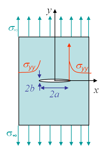
Let us analyze the case of a hole in an infinite plate submitted to uniform traction. Ingis modeled this case by solving the case of an ellipsoidal void (1913), see Picture I.50.
\begin{equation} \sigma_\text{max} = \sigma_{yy}\left(a,0\right) = \sigma_\infty \left(1+\frac{2a}{b}\right). \label{eq:sigmamax} \end{equation}
The case of a crack can be recovered by taking $b \rightarrow 0$. In that case $\sigma_\text{max}$ tends to infinity at the crack tip, meaning that if one wants to limit the stress value to a threshold, as when designing to remain in the elastic regime, $\sigma_\infty$ needs to tend to 0. However Griffith and Irwin have shown that a sample with a crack can still sustain a loading:
\begin{equation} \sigma_{\text{TS}}\sqrt{a} \div \sqrt{E\left(2\gamma_s+W_\text{pl}\right)}. \label{eq:irwin} \end{equation}
In order to solve the contradiction between the stress analysis and the experimental observations, fracture mechanics was developed to answer to the following questions:
- For a sample with an existing crack, knowing the crack size, what is the maximum loading leading to crack propagation?
- For a sample with an existing crack submitted to a cyclic loading, if the stress remains lower than the fracture stress, what is the life of the structure?
In this overview we will first consider the case of linear elastic materials. Note that this assumption will not always hold, but we will discuss this in details later on.
Linear Elastic Fracture Mechanics (LEFM)
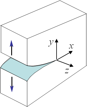
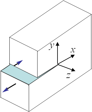
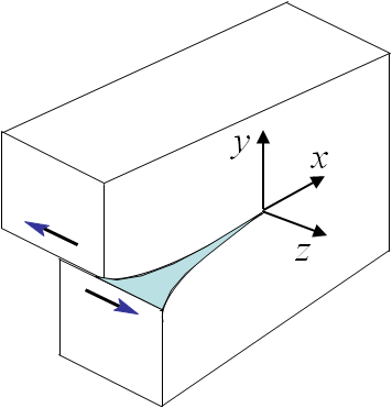
Under this assumption, the laws of mechanics for elastic linear materials can directly be used. In order to solve the problem of a sample with a crack, Irwin has studied three different loading modes. There are two modes loading the crack in its plane, the Mode I also called opening mode as it tends to open the crack lips, see Picture I.51, and the Mode II also called sliding mode as it tends to make the two crack lips slide on each other, see Picture I.52. The Mode III, also called shearing mode, loads the crack out of its plane, see Picture I.53.
Asymptotic solution
\begin{equation}\begin{cases} \mathbf{\sigma}_{zz} = 0\text{ or } \mathbf{\varepsilon}_{zz} = 0 \\ \mathbf{\sigma}_{yy}(\theta \pm \pi) = 0 \\ \mathbf{\sigma}_{xy}(\theta \pm \pi) = 0 \\ \mathbf{u}_x (\theta) = \mathbf{u}_x (-\theta) \\ \mathbf{u}_y (\theta) = -\mathbf{u}_y (-\theta) \end{cases},\label{eq:bcModeI}\end{equation} |
\begin{equation}\begin{cases} \mathbf{\sigma}_{zz} = 0\text{ or } \mathbf{\varepsilon}_{zz} = 0 \\ \mathbf{\sigma}_{yy}(\theta \pm \pi) = 0 \\ \mathbf{\sigma}_{xy}(\theta \pm \pi) = 0 \\ \mathbf{u}_x (\theta) = -\mathbf{u}_x (-\theta) \\ \mathbf{u}_y (\theta) = \mathbf{u}_y (-\theta) \end{cases},\label{eq:bcModeII}\end{equation} |
\begin{equation}\begin{cases} \mathbf{\sigma}_{xx} = \mathbf{\sigma}_{xy} = 0 \\ \mathbf{\sigma}_{yy} = \mathbf{\sigma}_{zz} = 0 \\ \mathbf{u}_x = \mathbf{u}_y = 0 \\ \mathbf{u}_z (\theta) = -\mathbf{u}_z (-\theta) \end{cases}.\label{eq:bcModeIII}\end{equation} |
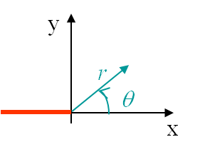
Classical solid mechanics can be applied on each of these modes in order to compute the stress and strain field. To do so the polar coordinates linked to the crack tip will be used, see Picture I.54. The only things that differentiate the three modes are the boundary conditions of the problem, which can directly be written in terms of the polar coordinates as (\ref{eq:bcModeI}-\ref{eq:bcModeIII}). Once the boundary conditions are known, it is possible to solve the problem. The calculations will be presented in details in the next lecture, but we can already discuss the results. The solution is obtained as series in $\sqrt{r}$, where $r$ is the distance to the crack tip, see Picture I.54, and reads for Mode I:
\begin{equation} \begin{cases} \sigma_{xx} = \frac{C}{\sqrt{r}}\cos{\frac{\theta}{2}}\left[1-\sin{\frac{3\theta}{2}}\sin{\frac{\theta}{2}}\right]+\mathcal{O}\left(r^0\right)\\ \boxed{\sigma_{yy} = \frac{C}{\sqrt{r}}\cos{\frac{\theta}{2}} \left[1+\sin{\frac{3\theta}{2}}\sin{\frac{\theta}{2}}\right]}+\mathcal{O}\left(r^0\right)\\ \sigma_{xy} = \frac{C}{\sqrt{r}}\cos{\frac{\theta}{2}} \cos{\frac{3\theta}{2}}\sin{\frac{\theta}{2}}+\mathcal{O}\left(r^0\right)\\ \mathbf{u}_x = \frac{C\left(1+\nu\right)}{E}\sqrt{r}\cos{\left(\frac{\theta}{2}\right)}\left[\kappa-1+2\sin^2\left(\frac{\theta}{2}\right)\right]+\mathcal{O}\left(r\right)\\ \mathbf{u}_y = \frac{C\left(1+\nu\right)}{E}\sqrt{r}\sin{\left(\frac{\theta}{2}\right)}\left[\kappa+1-2\cos^2\left(\frac{\theta}{2}\right)\right]+\mathcal{O}\left(r\right) \end{cases},\label{eq:solModeI}\end{equation}
where $\kappa$ is an expression of the Poisson ratio $\nu$ and is equal to $3-\nu \over 1+\nu$ for the plane stress state and to $3-4\nu$ for the plane strain state. For Mode II one can find a similar solution:
\begin{equation}\begin{cases} \mathbf{\sigma}_{xx} = - \frac{C}{\sqrt{r}}\sin{\frac{\theta}{2}}\left[2+\cos{\frac{3\theta}{2}}\cos{\frac{\theta}{2}}\right]+\mathcal{O}\left(r^0\right)\\ \mathbf{\sigma}_{yy} = \frac{C}{\sqrt{r}}\cos{\frac{\theta}{2}} \sin{\frac{\theta}{2}}\cos{\frac{3\theta}{2}}+\mathcal{O}\left(r^0\right)\\ \boxed{\mathbf{\sigma}_{xy} = \frac{C}{\sqrt{r}}\cos{\frac{\theta}{2}}\left[1-\sin{\frac{3\theta}{2}}\sin{\frac{\theta}{2}}\right]}+\mathcal{O}\left(r^0\right)\\ \mathbf{u}_x = \frac{C\left(1+\nu\right)}{E}\sqrt{r}\sin{\left(\frac{\theta}{2}\right)}\left[\kappa+1+2\cos^2\left(\frac{\theta}{2}\right)\right]+\mathcal{O}\left(r\right)\\ \mathbf{u}_y = -\frac{C\left(1+\nu\right)}{E}\sqrt{r}\cos{\left(\frac{\theta}{2}\right)}\left[\kappa-1-2\sin^2\left(\frac{\theta}{2}\right)\right]+\mathcal{O}\left(r\right)\end{cases}.\label{eq:solModeII}\end{equation}
Finally, for Mode III the solution reads:
\begin{equation}\begin{cases} \mathbf{\sigma}_{xz} = -\frac{C}{\sqrt{r}}\sin{\frac{\theta}{2}}+\mathcal{O}\left(r^0\right)\\ \boxed{\mathbf{\sigma}_{yz} = \frac{C}{\sqrt{r}}\cos{\frac{\theta}{2}}}+\mathcal{O}\left(r^0\right)\\ \mathbf{u}_z = \frac{4C\left(1+\nu\right)}{E}\sqrt{r}\sin{\left(\frac{\theta}{2}\right)}+\mathcal{O}\left(r\right)\end{cases}.\label{eq:solModeIII}\end{equation}
Let us first consider a mode I loading and let us analyze the dominant term of $\mathbf{\sigma}_{yy}$ (\ref{eq:solModeI}), which is the stress field characterizing the stress concentration of a plate under tension, see Picture I.50. Clearly the dominant term near the crack tip is in $\frac{C}{\sqrt{r}}$, meaning there is a singularity at the crack tip. Thus the value of the stress cannot be used to determine whether the crack will propagate or not. The idea of Irwin was thus to consider "how fast the stress tends to infinity" near the crack tip. To do so he has defined the stress intensity factor (SIF) to circumvent the singularity of the solution:
\begin{equation}\begin{cases} K_I =\lim_{r\rightarrow 0} \left(\sqrt{2\pi r} \mathbf{\sigma}^{\text{mode I}}_{yy}\left.\right|_{\theta=0}\right)= C\sqrt{2\pi} \\ K_{II} =\lim_{r\rightarrow 0} \left(\sqrt{2\pi r} \mathbf{\sigma}^{\text{mode II}}_{xy}\left.\right|_{\theta=0}\right)= C\sqrt{2\pi} \\ K_{III} =\lim_{r\rightarrow 0} \left(\sqrt{2\pi r} \mathbf{\sigma}^{\text{mode III}}_{yz}\left.\right|_{\theta=0}\right)= C\sqrt{2\pi} \end{cases}.\end{equation}
In this equation we have also treated the two other fracture modes by considering the dominant stress terms of mode II (\ref{eq:solModeII}) and of mode III (\ref{eq:solModeIII}). For a given loading mode, this SIF, expressed in $\text{MPa}\cdot \sqrt{\text{m}}$, characterizes the stress evolution near the crack tip:
\begin{equation}\begin{cases} \mathbf{\sigma}^\text{mode i} = \frac{K_i}{\sqrt{2\pi r}} \mathbf{f}^\text{mode i}(\theta) \\ \mathbf{u}^\text{mode i} = K_i\sqrt{\frac{r}{2\pi}} \mathbf{g}^\text{mode i}(\theta) \end{cases},\label{eq:fandg}\end{equation}
where $\mathbf{f}$ and $\mathbf{g}$ are functions defined for each mode but independent of the loading and geometry (as long as we consider the asymptotic value). The loading and geometry effects are thus fully reported to the value of the SIF. Irwin has thus the idea to consider the value of the SIF to detect the crack propagation. Indeed experiments have shown that for a given material, which obeys to the LEFM assumption, the crack propagates if the SIF reaches a threshold $K_C$ called the toughness of the material.
Crack propagation criterion and toughness
From the previous section, one can write the crack propagation criterion in mode I as:
\begin{equation}K_I\quad\begin{cases} < K_{IC} \rightarrow \text{ the crack does not propagate,}\\ \geq K_{IC} \rightarrow \text{ the crack does propagate,} \end{cases}\label{eq:SIFCriterion}\end{equation}
where $K_{IC}$ is the mode I toughness. Remember, under the LEFM assumption:
- $K_I$ depends on the geometry and loading conditions only,
- $K_{IC}$ depends on the material only.
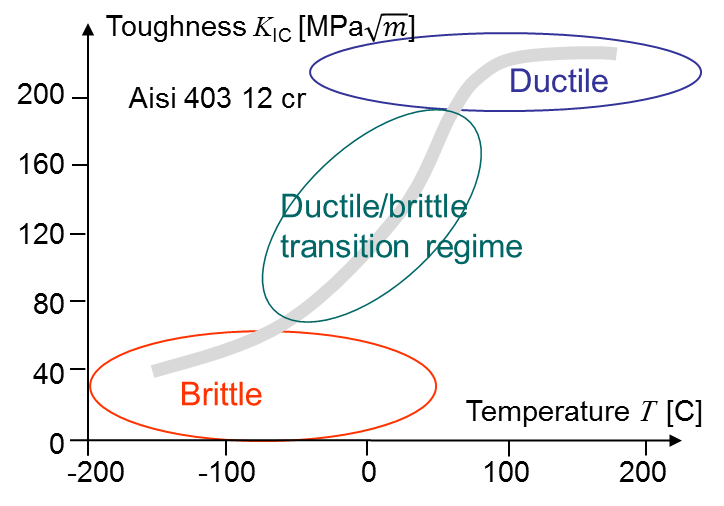
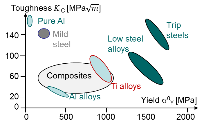
Orders of magnitude for the toughness are for example for concrete 0.2-1.4 $\text{MPa}\cdot\sqrt{\text{m}}$ and typical values for other materials are reported in Picture I.55. Materials for which the toughness is lower than 30 to 40 $\text{MPa}\cdot\sqrt{\text{m}}$ are considered as brittle materials. Ductile materials have a higher toughness, but as we will discuss it in length later they usually do not satisfy to the LEFM assumption as their behavior is no longer elastic. As discussed before, some materials have a brittle behavior at low temperature and a ductile behavior at high temperature. For such materials the toughness depends on the temperature and there exists a transition region as shown in Picture I.56. Note that at high stress rate these materials also loose ductility.
Evaluation of the SIFs
The next question which arises is "How do we can determine this SIF" that has to be compared to the material toughness. As said, this SIF depends on the geometry and on the loading condition. In practice, there exist 5 different methods.
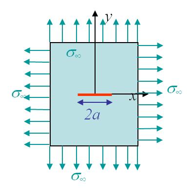
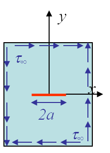
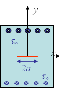
- Analytical method. This can only be achieved for simple cases as for a crack of size 2a in an infinite plate as shown in Picture I.57, I.58 and I.59. In these cases the following analytical results for the different SIFs can be computed as it will be done in the next lecture:
- Superposition principle. As the problem is fully linear, we can apply the superposition principle. Note that one can add the SIFs related to the same mode only. Indeed according to (\ref{eq:fandg}), the functions $\mathbf{f}$ and $\mathbf{g}$, which depend on θ, are different for the different modes. Thus adding the stress tensor (by superposition principle) does not correspond to adding the SIFs of different modes. Thus for two different loadings $a$ and $b$ we have $K_i = K_i^a + K_i^b$, but for two different modes, we have $K \ne K_I + K_{II}$ !
- Use of handbooks. Solutions for different (simple) geometries obtained by different ways are tabulated in handbooks.
- Finite Element (FE) method. We will extensively describe how to determine the SIFs from a FE resolution.
- Energetic approach. This method makes the bridge between the work of Griffith based on the fracture energy and the asymptotic solution. We will introduce this point briefly here below, but a complete lecture is dedicated to it.
\begin{equation}\begin{cases} K_I = \sigma_\infty \sqrt{\pi a} \\ K_{II} = \tau_\infty \sqrt{\pi a} \\ K_{III} = \tau_\infty \sqrt{\pi a} \end{cases}.\label{eq:SIFinf}\end{equation}
For more complicated problems, the SIFs cannot be computed in a closed-form, but they follow
\begin{equation}\begin{cases} K_I = \beta_{I}\sigma_\infty \sqrt{\pi a} \\ K_{II} = \beta_{II}\tau_\infty \sqrt{\pi a} \\ K_{III} = \beta_{III}\tau_\infty \sqrt{\pi a} \end{cases},\end{equation}
where the $\beta_i$ are now values that depend on the geometry and on the crack size.
Measurement of the toughness
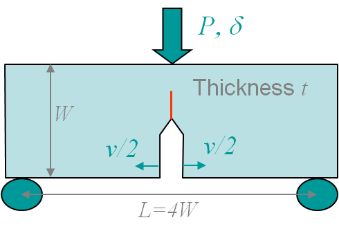
Once the SIFs of a structure are computed, they have to be compared to the toughness of the material. This value has to be measured experimentally by strictly following the procedure defined by the ASTM E399 Standard. Different kinds of samples can be manufactured from a given material as the Single Edge Notched Bend (SENB) specimen as shown in Picture I.60. To remain conservative, it is necessary to be in the plane strain state (P-$\varepsilon$), which means that the specimen is thick enough (a quantity yet to be defined). Indeed in the plane stress state (P-$\sigma$) the measured toughness is higher as it will be explained later on. The specimen has initially a V-notch, which will initiate the crack. The evaluation of the toughness requires the following steps
- Calibrate the measurement technics of the three-point bending test to measure the evolution of the displacement $\delta$ and of the crack-mouth opening $\nu$ in terms of the loading force $P$.
- Initiate an initial crack by fatigue by applying a cyclic loading well below the fracture loading.
- Measure the compliance $\frac{\nu}{P}$ of $\frac{\delta}{P}$ of the cracked specimen and determine the value $a$ of the crack using FE predictions $\frac{\nu}{P}=f\left(a\right)$.
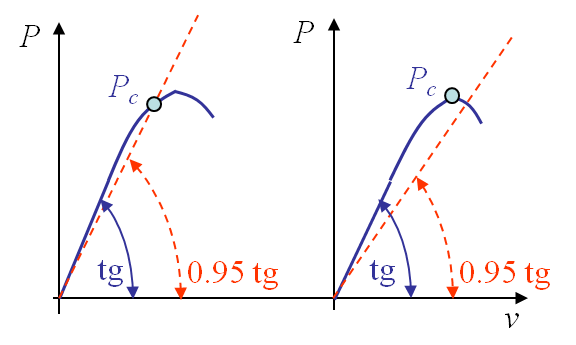
- Perform the three-point bending test to measure the critical loading $P_C$. This value is obtained using the experimental P-$\nu$ loading curve, see Picture I.61. $P_C$ is defined as the loading value obtained for a 95%-offset of the initial structural stiffness. However if the maximum value of P is reached before this offset, this corresponds to the critical value $P_C$.
- The toughness is then deduced using the expression of the SIF obtained from FE simulations:
\begin{equation} K_I = \frac{PL}{t W^{\frac{3}{2}}} f\left(\frac{a}{W}\right), \label{eq:SIFToughness}\end{equation}
where $\frac{a}{W}$ depends on the test specimen (SENB ...). Substituting $P_C$ in (\ref{eq:SIFToughness}) directly gives $K_{IC}$.
Relation with the fracture energy
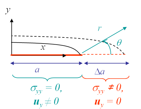
In the previous subsection we have seen how to determine whether a crack will propagate or not. However in the last section we have seen that the critical crack size is related to the fracture energy. This topic will be extended in a coming lecture, but we can already get some insight of the phenomenon by considering a Mode I loading of a $2a$-long centered crack in an infinite plate. Considering the polar coordinates at one of the two crack tips (before crack propagation), see Picture I.62, the stress and displacement fields ahead of the crack tip are deduced from (\ref{eq:solModeI}-\ref{eq:SIFinf}) by considering $\theta=0$ and $x=r+a$, leading to:
\begin{equation}\begin{cases} \mathbf{\sigma}^0 (\theta=0,\,r=x-a) = \frac{\sigma_\infty \sqrt{a}}{\sqrt{2 (x-a)}} \\ \mathbf{u}^0_y (\theta=0,\,r=x-a) = 0 \end{cases}.\label{eq:ene1}\end{equation}
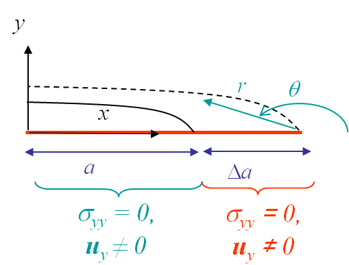
Now we consider that the crack has grown straight ahead to reach a size $2(a + \Delta a)$, see Picture I.63. The part of the crack lips which now corresponds to the increment $\Delta a$ was before a sound material with the stress and displacement fields (\ref{eq:ene1}). This part corresponds now to opened crack lips, and the displacement and stress fields of the upper/lower crack lip can still be deduced from (\ref{eq:solModeI}-\ref{eq:SIFinf}), but this by considering $\theta \rightarrow \pm\pi$ and $x=a+\Delta a -r$, leading to:
\begin{equation}\begin{cases} \mathbf{\sigma}_{yy}^1 \left(\theta=\pi,\,r=a+\Delta a- x\right) &= 0 \\ \mathbf{u}^1_{y}\left(\theta=\pm\pi,\,r=a+\Delta a - x\right) &= \pm\frac{\sigma_\infty\left(1+\nu\right)\left(\kappa+1\right)}{E\sqrt{2}}\\&\sqrt{a+\Delta a}\sqrt{a+\Delta a -x} \end{cases}.\label{eq:ene2}\end{equation}
From (\ref{eq:ene1}) and (\ref{eq:ene2}), we can see that the part of interest is subjected to a stress field $ \mathbf{\sigma}_{yy}^0$ but at zero-displacement before the crack propagation, while it is subjected to an opening displacement $\mathbf{u}^1_{y}$ but is stress-free after crack propagation. There is thus an energy released by the structure as the stress tensor exhibits a work during the crack propagation. This energy can be computed as:
\begin{equation} \Delta E_{\text{int}} = -4dz \int_a^{a+\Delta a} \int_{\mathbf{u}_y^0}^{\mathbf{u}_y^1} \mathbf{\sigma}_{yy} d \mathbf{u}_y dx,\label{eq:eneReleased} \end{equation}
where the factor 4 comes from the fact that there is double symmetry around the x and y axes (Remembering that there is a crack increment of size $\Delta a$ on each side of the centered crack). As we consider a linear elastic material, during the crack opening $\mathbf{\sigma}_{yy}$ has to decrease linearly with the displacement $\mathbf{u}_y$, and the integral over the displacement can be easily be solved leading to:
\begin{equation} \Delta E_{\text{int}} = -2 dz \int_a^{a+\Delta a} \mathbf{\sigma}^0_{yy}\mathbf{u}^1_y dx. \end{equation}
Using the values (\ref{eq:ene1}-\ref{eq:ene2}), and applying the change of variables $x=a+\Delta a \cos^2\theta$, the energy released reads:
\begin{equation} \Delta E_{\text{int}} = -\frac{dz \sigma_\infty^2 \sqrt{a\left(a+\Delta a\right)}\left(1+\nu\right)\left(1+\kappa\right)}{2E}\pi\Delta a. \end{equation}
If we relate this energy to the increment of crack surface $dA=2\Delta a dz$ and change the sign as to have a positive value, we have an important concept for fracture mechanics, which is the energy release rate $G$:
\begin{equation} G=-\frac{d E_{\text{int}}}{d A}.\label{eq:G} \end{equation}
This energy corresponds to the energy released by the structure by unit increment of the crack surface. It reads in our case:
\begin{equation} G=-\frac{d E_{\text{int}}}{d A}= -\lim_{\Delta a\rightarrow 0}\frac{\Delta E_{\text{int}}}{2 \Delta a dz}= \frac{\pi a \sigma_{\infty^2}}{4E}\left(1+\nu\right)\left(\kappa+1\right)=\frac{\pi a \sigma_{\infty^2}}{E'}=\frac{K^2_I}{E'},\label{eq:Ginf} \end{equation}
where
\begin{equation} E'=\frac{4E}{\left(1+\nu\right)\left(\kappa+1\right)}=\left\{ \begin{array}{ll} E & \text{Plane stress state} \\ \frac{E}{1-\nu^2} & \text{Plane strain state} \end{array} \right. .\end{equation}
In this example we have assumed a crack lying in an infinite plate. In the next lectures, it will be showed that for a crack propagating straight ahead under mode I we always have under the LEFM assumption
\begin{equation} G=\frac{K^2_I}{E'}. \end{equation}
We will also see later than as the energies can be added, we get for the global energy release rate, not forgetting the assumption of a straight forward growing crack:
\begin{equation} G=\frac{K^2_I}{E'}+\frac{K^2_{II}}{E'}+\frac{\left(1+\nu\right)K^2_{III}}{E} \end{equation}
This expression relates the SIFs to the energy that the structure releases when a crack propagates. This is a first link between the energy and the stress approaches. Going further on with the energy approach, we can follow Griffith (1920) approach. The total energy of the specimen can be seen as the sum of the internal (elastic) energy $E_\text{int}$ with the energy $\Gamma$ needed to create a crack of surface $A$ :
\begin{equation} E=E_\text{int} + \Gamma \end{equation}
Deriving this equation with respect to the crack surface $A$ and considering that the total energy is conserved (as no dissipation is considered) yields:
\begin{equation} \frac{\partial E}{\partial A} = \frac{\partial E_{\text{int}}}{\partial A} + \frac{\partial \Gamma}{\partial A}=0.\label{eq:derEnergy} \end{equation}
Using the definition of the energy release rate (\ref{eq:G}), this last equation leads to
\begin{equation} G=-\frac{dE_{\text{int}}}{dA}=\frac{d\Gamma}{dA}.\end{equation}
Assuming the crack is actually growing, the term $\frac{d\Gamma}{dA}$ actually corresponds to twice the surface energy $\gamma_s$ by definition of the surface energy (and as we form two surfaces $A$). Thus the former equation reads
\begin{equation} G=-\frac{dE_{\text{int}}}{dA}=\frac{d\Gamma}{dA} =2 \gamma_s= G_c. \label{eq:Gc}\end{equation}
The meaning of this equation is the following. For a crack to grow the energy that the structure would have to realease due to the crack growth (by unit crack surface) have to be larger or equal to $G_C$ the energy required to form a crack (of unit surface). For brittle material this is twice the surface energy and corresponds to the energy required to have cleavage. As we said that the crack would grow if $K_I\geq K_{IC}$, the crack would grow if $G \geq G_c$.
Assuming the crack does propagate, then combining (\ref{eq:Ginf}), in which we substitute $\sigma_\infty$ by the strength of the material $\sigma_{\text{TS}}$, with (\ref{eq:Gc}) leads to
\begin{equation} \sigma_{\text{TS}}=\sqrt{\frac{2\gamma_s E}{\pi a}}, \end{equation}
which is nothing else than the Griffith formula for brittle materials seen before.
Let us now consider the practical implication of this formula:
- For glass ($2\gamma_s =$ 2 J / m2 and $E =$ 60 GPa): $\sigma_{\text{TS}}\sqrt{a} = 195 \text{kPa m}^{\frac{1}{2}}$
- For mild steel at room temperature (ductile plastic work will be dominating, $2\gamma_s =$ 200 kJ / m2 and $E =$ 210 GPa):$\sigma_{\text{TS}}\sqrt{a} = 115 \text{MPa m}^{\frac{1}{2}}$
This example shows how ductile materials have a much higher tensile strength for the same crack size, explaining the troubles of the liberty ships.
Direction of crack propagation
We have determined whether a crack grows when loaded in mode I. In that case, by symmetry the crack propagates straight ahead. What would happen when the loading mode is mixed (for example a combination of mode I and mode II)?
- What is the condition for crack growth?
- In which direction would it grow?
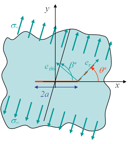
To answer to these questions, let us consider the mixed mode loading of Picture I.64, in which the loading direction is oriented with an angle $\beta^*$ with respect to the crack ($\beta^*=\frac{\pi}{2}$ corresponding to a pure mode I loading). As it will be demonstrated later, the SIFs of the two modes can be related from:
\begin{equation} \cot\beta^\star = \frac{K_{II}}{K_I}. \end{equation}
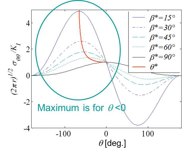
One assumption to define the direction of the crack growth is to state that the crack grows in the direction so that the SIF related to Mode I in the new frame is maximum. This actually corresponds to maximizing $\mathbf{\sigma}_{yy}$ in this new frame, i.e. it corresponds to maximizing the hoop stress $\sigma_{\theta\theta}$ in the orginal polar coordinates. This latter can be computed as (this will be demonstrated later):
\begin{equation} \mathbf{\sigma}_{\theta\theta} = \frac{K_I}{\sqrt{2\pi r}}\left[\cos^3{\frac{\theta}{2}} - \frac{3\cot{\beta_\star}}{2}\sin{\theta}\cos{\frac{\theta}{2}}\right] \label{eq:hoop}.
\end{equation}
The direction $\theta^\star$ of the maximum hoop stress is thus given by:
\begin{equation} \partial_\theta \mathbf{\sigma}_{\sigma\sigma}|_{\theta^\star} = 0, \label{eq:maxhoop}\end{equation}
and the crack growth criterion (which is thus mode I in that direction) becomes
\begin{equation} \left(\sqrt{2\pi r}\mathbf{\sigma}_{\theta\theta}\left(r,\,\theta^\star\right)\right) \geq K_{IC}. \label{eq:hoopKC}\end{equation}
Picture I.65 shows the evolution of the stress $\sigma_{\theta\theta}$ (\ref{eq:hoop}) with respect to the angle $\theta$ and different mixed loading cases $\beta^*$. The direction of the maximum hoop stress is also reported as a red curve. What can be seen is that for a positive loading angle, the crack will kink with a negative angle.
J-integral
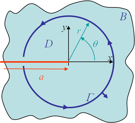
As explained previously the concept of crack propagation is strongly linked to the energy released during crack propagation. One practical way to compute the energy, without requiring the crack to actually grow, is the J-integral introduced by Rice. The J-integral corresponds to the energy flowing through a contour embedding the crack tip as shown in Picture I.64, and reads
\begin{equation} J = \int_\Gamma \left[ U(\varepsilon) \mathbf{n}_x - \partial_x \mathbf{u} \cdot \mathbf{T} \right] dl,\label{eq:Jint} \end{equation}
in which the first term corresponds to the flow parallel to the crack of the material energy and the second term to the flow parallel to the crack of the traction energy on the contour (as $\mathbf{T}=\mathbf{\sigma}\cdot\mathbf{n}$ and as $\mathbf{n}$ is the outward unit normal of the contour).
The J-integral has the following properties:
- It is path independent if the contour Γ embeds a straight crack tip;
- There is no assumption on how the crack will grow;
- If the crack grows straight ahead, $J = G$;
- If the sample is linear elastic, $J = \frac{K_I^2}{E'} + \frac{K_{II}^2}{E'} + \frac{K_{III}^2}{2\mu} $;
- The J integral can be extended to plasticity when unloading is prohibited.
Because of these properties, the J-integral is:
- An efficient numerical tool to evaluate the SIFs in FE simulations;
- Useful for non-perfectly brittle materials.
We will expend the concept of the J-integral in a coming lecture.
Case of ductile materials
In the case of ductile materials, two more aspects need to be considered.
Resistance curve and crack stability
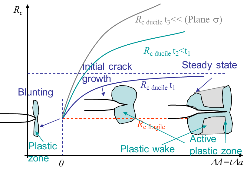
We have seen in (\ref{eq:Gc}) that a crack propagates if $G \geq G_C$. For a perfectly brittle material the fracture energy is constant and equal to $2\gamma_s$. For other materials there will be a plastic flow at the crack tip as a stress cannot physically reach the infinity as predicted by the LEFM approach. This plastic flow arises in the active plastic zone as illustrated in Picture I.67. Evidently this active plastic zone moves with the crack tip in case of crack growth, meaning that the crack is opening in a zone affected by permanent plastic deformations: the plastic wake. This makes the crack more difficult to be opened, which corresponds to an increase of the apparent fracture energy $G_C$ with the crack propagation $\Delta a$. This is call the resistance and $G_c$ is replaced by $R_c(a)$. Some material can have a steady-state in the resistance curve as in Picture I.67, other not. Note that the curve does not only depend on the material, but also on the geometry as the thickness.
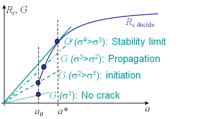
During the crack propagation the geometry of the structure changes (as the crack changes) so does the energy release rate $G$. Assuming a constant force loading, $G$ increases with the crack length at it will be shown later. On the one hand, for a perfectly brittle material as $G_C$ is constant, once the crack initiates it keeps propagating as $G$ remains larger than the constant $G_C$. On the other hand, for a ductile material $R_c$ also evolves with the crack size and a crack can now be stable. This is illustrated in Picture I.68. Assuming an initial crack size $a_0$, the crack propagates if the loading reach $\sigma=\sigma_2$. However under this loading condition, for a crack size $a_0+ \Delta a$, $G\left(\sigma_2,\, a_0+ \Delta a\right)<R_C\left(a_0+ \Delta a\right)$ and the crack stops. To make the crack growth one has to increase the loading up to $\sigma_3$ but the crack would also eventually stop: the crack is stable. This behavior changes if the loading reaches $\sigma_4$ as in this case $G$ is always larger than $R_C$ for any crack size $a$: the crack is unstable. Mathematically, this reads:
A crack is stable if $G = R_c\left(a\right)$ and $\frac{dG}{da} \leq \frac{d R_c}{da}$, or unstable if $G = R_c\left(a\right)$ and $\frac{dG}{da} > \frac{d R_c}{da}$.
LEFM limit
We have just considered ductile materials, which exhibit plastic deformations. However up to now we have considered the LEFM approach which assumes elastic linear materials. The validity of the method is thus questionable.
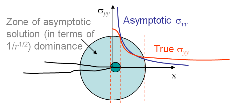
Let us first assume there are no plastic deformations. The LEFM asymptotic method thus predicts a stress field in $\frac{1}{\sqrt{r}}$ tending to infinity at the crack tip, see Picture I.69. This is of course unphysical and some irreversible behaviors occur near the crack tip (dark green zone on Picture I.69). The asymptotic solution is thus not valid in this zone. Now faraway of the crack tip, the asymptotic solution has neglected the terms in $r^0$, $\sqrt{r}$, $r$ ... and does not capture the structural response (faraway from the crack tip the asymptotic solution predicts a stress tending to zero, which is not usually the correct answer), see Picture I.69. As a summary, the LEFM solution is not valid faraway from the crack tip and is not valid close to the crack tip in a zone whose size depends on the degree of plastic deformations involved.
- For some materials, considered as brittle, if the sample is large enough the dark green zone of Picture I.69 remains small enough and there exists a cylindrical zone (light green in Picture I.69), in which the asymptotic solution if valid. In this case the LEFM approach can be used.
- If the material is more ductile, or if the sample is too small, the dark green region becomes bigger with respect to the structural response stress field zone and the region of validity of the asymptotic solution vanishes. LEFM approach cannot be used anymore.
In coming lectures we will see how to validate the applicability of the LEFM approach and also consider Non-Linear Fracture Mechanics (NLFM) when required.
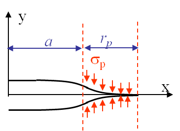
If the crack front plastic zone $r_p$ remains smaller but is of comparable order of magnitude with respect to the crack length $a$, see Picture I.70, the LEFM approximation still holds (i.e. there exists a region of validity as in Picture I.69) and we are typically under the Small Scale Yielding assumption (SSY). A first order correction can be achieved to improve the accuracy of the method: when determining the SIFs one needs to replace the crack length by the effective crack length $a_\text{eff}$, which accounts for the blunting in the plastic zone, see Picture I.70. The system of equations to be solved reads:
\begin{eqnarray} a \rightarrow a_{\text{eff}} & = & a +\frac{r_p}{3} \\ r_p & = & \frac{\pi K^2_I\left(a_\text{eff}\right)}{8\sigma_p^2} \end{eqnarray}
When the plastic zone becomes too large, when the applied stress is larger than half the yield stress of the material, none of the discussed approximations hold and it is necessary to use the NLFM approach.
![]()