
\(\newcommand{\cauchy}{\boldsymbol{\sigma}}\) \(\newcommand{\strain}{\boldsymbol{\varepsilon}}\) \(\newcommand{\uV}{\boldsymbol}\) \(\newcommand{\uT}{\mathbf}\) \(\newcommand{\defu}{\boldsymbol{u}}\)
HRR theory > Semi-infinite mode I crack in plane-$\varepsilon$ state
In the previous section, we have derived an asymptotic expression of the stress and strain fields in terms of the $J$-integral. In this section, we will use the Airy function and the stream function to derive the stress and strain components tensors for a semi-infinite mode I crack in plane-$\varepsilon$ state.
Resolution for a semi-infinite crack in plane-$\varepsilon$ state
Stress field: Airy functions
Similarly to linear elastic fracture mechanics, for an arbitrary body, the general linear equation for the balance of momentum, in index form, is
\begin{equation} \rho \ddot{\uV{x}}_\alpha = \uV{b}_\alpha + \cauchy_{\alpha\beta,\beta}\,, \end{equation}
where $\uV{b}_i$ contains the volume forces. In the static case and in the absence of body forces, the stress tensor can be expressed through an Airy function $\Phi$, which is a scalar, by
\begin{equation} \cauchy_{\alpha\beta} = - \Phi_{,\alpha\beta} + \delta_{\alpha\beta} \Phi_{,\gamma\gamma} \, \text{.} \label{eq:AiryStressCart}\end{equation}
Indeed, the linear momentum equation becomes
\begin{equation} \cauchy_{\alpha\beta,\beta} = - \Phi_{,\alpha\beta\beta} + \delta_{\alpha\beta} \Phi_{,\gamma\gamma\beta}= 0 \, \text{.} \end{equation}
However, contrarily to the LEFM asymptotic solution derivation, since we are not in linear elasticity, the Hooke's law does not apply and the double Laplacian of the Airy function is not zero anymore
\begin{equation} \nabla^2 \nabla^2 \Phi \neq 0 \, \text{.} \end{equation}
Also in the same way as derived in Lecture 2, the stress tensor (\ref{eq:AiryStressCart}) can be stated in polar coordinates following
\begin{equation}\label{eq:stress_Airy} \begin{cases} \mathbf{\sigma}_{rr} = \frac{1}{r}\Phi_{,r}+\frac{1}{r^2}\Phi_{,\theta\theta}\,, \\ \mathbf{\sigma}_{\theta\theta} = \Phi_{,rr}\,, \\ \mathbf{\sigma}_{r\theta} = -\frac{1}{r}\Phi_{,r\theta}+\frac{1}{r^2}\Phi_{,\theta} \, \text{.} \end{cases} \end{equation}
When considering the asymptotic solution, since we are seeking a solution in $r^{-1/(n-1)}$, a suitable choice for the Airy function would be
\begin{equation} \Phi = \frac{\left(n+1\right)^2}{n\left(2n+1\right)} r^{\frac{2n+1}{n+1}} f\left(\theta\right) \, \text{.}\label{eq:StreamPhi} \end{equation}
where $f\left(\theta\right)$, a function independent from $r$, has yet to be defined. Derivating the Airy function and inserting the outcome in (\ref{eq:stress_Airy}) results in
\begin{equation} \begin{cases} \cauchy_{rr}= r^{\frac{-1}{n+1}}\left(\frac{n+1}{n} f+\frac{\left(n+1\right)^2}{n\left(2n+1\right)}f'' \right)\,, \\ \cauchy_{\theta\theta}= r^{\frac{-1}{n+1}} f\,, \\ \cauchy_{r\theta}= r^{\frac{-1}{n+1}}\left(- \frac{n+1}{n} + \frac{\left(n+1\right)^2}{n\left(2n+1\right)} \right)f'=r^{\frac{-1}{n+1}} \frac{-\left(n+1\right)} {\left(2n+1\right)}f' \,.\end{cases}\label{eq:stressFromF} \end{equation}
Strain field: Stream functions
In order to evaluate the strain field, the stream functions can be utilized. Indeed, the strain components in plane-$\varepsilon$ state are given by the derivatives of the displacement following
\begin{equation} \begin{cases} \strain_{\alpha\beta}=\frac{\defu_{\alpha,\beta}+\defu_{\beta,\alpha}}{2}\,, \\ \strain_{zz} = 0 \, \text{.} \end{cases} \end{equation}
However, since the material is assumed to be incompressible, the strain components in plane-$\varepsilon$ satisfy
\begin{equation} 0= \strain_{ii}= \strain_{\alpha\alpha}=\defu_{\alpha,\alpha}\, \text{.} \label{eq:uncompressible} \end{equation}
The displacements thus derive from a stream function $\Psi$ with
\begin{equation} \begin{cases} \defu_x = \Psi_{,y}\,, \\ \defu_y = -\Psi_{,x} \,,\end{cases}\label{eq:uStream}\end{equation}
which satisfy Eq. (\ref{eq:uncompressible}). A change of variables in polar coordinates leads to
\begin{equation} \begin{cases} \defu_x = \Psi_{,y}=\sin{\theta}\Psi_{,r}+\frac{\cos{\theta}}{r}\Psi_{,\theta}\,, \\ \defu_y = -\Psi_{,x} = -\cos{\theta}\Psi_{,r}+\frac{\sin{\theta}}{r}\Psi_{,\theta} \, \text{,} \end{cases}\label{eq:uxuyFromPsi} \end{equation}
or again, using the rotation matrix $ \left(\begin{array}{cc} \cos{\theta} & \sin{\theta}\\ -\sin{\theta} & \cos{\theta} \end{array}\right) $, to the displacements field in polar coordinates
\begin{equation} \begin{cases} \defu_r= \cos{\theta}\defu_x +\sin{\theta}\defu_y = \frac{\Psi_{,\theta}}{r}\,, \\ \defu_\theta = -\sin{\theta}\defu_x +\cos{\theta}\defu_y = - \Psi_{,r}\,. \end{cases} \label{eq:uStreamPolar}\end{equation}
The strain tensor in polar coordinates then follows as
\begin{equation}\label{eq:strain_stream} \begin{cases} \strain_{rr}=\defu_{r,r}=\frac{\Psi_{,r\theta}}{r}-\frac{\Psi_{,\theta}}{r^2}\,, \\ \strain_{\theta\theta}=\frac{\defu_{r}}{r}+\frac{1}{r}\defu_{\theta,\theta}=-\strain_{rr}\,, \\ \strain_{r\theta}=\frac{1}{2}\left(\frac{\defu_{r,\theta}}{r}+\defu_{\theta,r}-\frac{\defu_\theta}{r}\right) = \frac{1}{2}\left(\frac{\Psi_{,\theta\theta}}{r^2}-\Psi_{,rr}+\frac{\Psi_{,r}}{r}\right) \, \text{.} \end{cases} \end{equation}
When considering the asymptotic solution, we are seeking a solution in $r^{-n/(n+1)}$ and an appropriate choice for the stream function would be
\begin{equation} \Psi = - r^{\frac{n+2}{n+1}} g\left(\theta\right) \,, \end{equation}
where $g\left(\theta\right)$, a function independent from $r$, has yet to be defined. Once again, inserting the derivatives of the stream function into (\ref{eq:strain_stream}), the individual strain components can be rewritten as
\begin{equation}
\begin{cases}
\strain_{rr}=\frac{\Psi_{,r\theta}}{r}-\frac{\Psi_{,\theta}}{r^2} = r^{\frac{-n}{n+1}} \left(-\frac{n+2}{n+1}g'+g'\right)=-\frac{1}{n+1} r^{\frac{-n}{n+1}} g'\,, \\
\strain_{\theta\theta}=\frac{1}{n+1} r^{\frac{-n}{n+1}} g' \,,\\
\strain_{r\theta}=\frac{1}{2}\left(\frac{\Psi_{,\theta\theta}}{r^2}-\Psi_{,rr}+\frac{\Psi_{,r}}{r}\right) =
\frac{r^{\frac{-n}{n+1}}}{2} \left(-g''+\frac{n+2}{\left(n+1\right)^2}g-\frac{n+2}{n+1}g \right) =
- \frac{r^{\frac{-n}{n+1}}}{2} \left(g''+ n \frac{n+2}{\left(n+1\right)^2}g \right) \, \text{.}
\end{cases}
\label{eq:strainFromF}\end{equation}
Power law and normal flow equation
In the derived stress and strain fields (\ref{eq:stressFromF}) and (\ref{eq:strainFromF}), the function $f\left(\theta\right)$ and $g\left(\theta\right)$ in terms of the angle $\theta$ have not been defined yet. Therefore, two equations are missing in order to close the system of equations. In particular these functions $f\left(\theta\right)$ and $g\left(\theta\right)$ have to satisfy, on the one hand the power law,
\begin{equation}\label{eq:powerLaw} \bar{\varepsilon} = \frac{\alpha \sigma_p^0}{E} \left( \frac{\sigma_e}{\sigma_p^0} \right)^n \end{equation}
as well as the normal flow equation
\begin{equation}\label{eq:normality} \strain = \bar{\varepsilon} \sqrt{\frac{3}{2}} \frac{\mathbf{s}}{\sqrt{\mathbf{s} \mathbf{s}}} = \frac{3\bar{\varepsilon}}{2\sigma_e} \mathbf{s} \, \text{.} \end{equation}
Equations resolution
By inserting the near-tip stress field (\ref{eq:stressFromF}) and strain field (\ref{eq:strainFromF}) in the power law (\ref{eq:powerLaw}) and in the normal flow (\ref{eq:normality}) equations, two $2^{\text{nd}}$ order ODEs in terms of the functions $f\left(\theta\right)$ and $g\left(\theta\right)$, and in $n$ are obtained, see details in the appendix, as follows
\begin{equation} \begin{cases} \left[\frac{4}{3\left(1+n\right)^2}g'^2+\frac{1}{3}\left(g''+n\frac{n+2}{\left(n+1\right)^2}g\right)^2\right] = \left(\frac{\alpha\sigma_p^0}{E\left(\sigma_p^0\right)^n}\right)^2\left[ \frac{3}{4}\left(\frac{1}{n} +\frac{\left(n+1\right)^2}{n\left(2n+1\right)}f''\right)^2+3\left(\frac{n+1}{2n+1}\right)^2f'^2\right]^n\,, \\ \frac{2}{2n+1}g'f' = -\frac{1}{2} \left[\frac{1}{n}f+\frac{\left(n+1\right)^2}{n\left(2n+1\right)}f''\right] \left[g''+n\frac{n+2}{\left(n+1\right)^2}g\right] \, \text{.} \end{cases}\label{eq:ODE1} \end{equation}
However, in order to extract the loading condition and geometry effect, as well as the dependency to the yield stress $\sigma_p^0$, we proceed as in the previous section, see the stress approximation and the strain approximation, by extracting the intensity factor $k_n$ and the yield stress $\sigma_p^0$. Similarly, the functions $f\left(\theta\right)$ and $g\left(\theta\right)$ can be expressed by
\begin{equation} \begin{cases} f\left(\theta\right) = \sigma_p^0 k_n \tilde{f}\left(\theta\right)\,, \\ g\left(\theta\right) = \frac{\alpha\sigma_p^0}{E}k^n_n \tilde{g}\left(\theta\right) \, \text{.} \end{cases}\label{eq:ftilde} \end{equation}
The near-tip stress field (\ref{eq:stressFromF}) and strain field (\ref{eq:strainFromF}) thus become
\begin{equation} \begin{cases} \cauchy_{rr}= r^{\frac{-1}{n+1}}\sigma_p^0 k_n\left(\frac{n+1}{n} \tilde{f}+\frac{\left(n+1\right)^2}{n\left(2n+1\right)}\tilde{f}'' \right)\,, \\ \cauchy_{\theta\theta}= r^{\frac{-1}{n+1}}\sigma_p^0 k_n \tilde{f}\,, \\ \cauchy_{r\theta}= r^{\frac{-1}{n+1}}\sigma_p^0 k_n \frac{-\left(n+1\right)} {\left(2n+1\right)}\tilde{f}' \,,\end{cases}\label{eq:stressFromFtilde} \end{equation}
and
\begin{equation} \begin{cases} \strain_{rr}=-\frac{1}{n+1} r^{\frac{-n}{n+1}}\frac{\alpha\sigma_p^0}{E}k^n_n \tilde{g}'\,, \\ \strain_{\theta\theta}=\frac{1}{n+1} r^{\frac{-n}{n+1}}\frac{\alpha\sigma_p^0}{E}k^n_n \tilde{g}' \,,\\ \strain_{r\theta}=- \frac{r^{\frac{-n}{n+1}}}{2} \frac{\alpha\sigma_p^0}{E}k^n_n\left(\tilde{g}''+ n \frac{n+2}{\left(n+1\right)^2}\tilde{g} \right) \, \text{.} \end{cases} \label{eq:strainFromFtilde}\end{equation}
Inserting (\ref{eq:ftilde}) in (\ref{eq:ODE1}) leads to two $2^{\text{nd}} $-order ODEs in terms of the non-dimensional functions $\tilde{f}$ and $\tilde{g}$
\begin{equation} \begin{cases} \left[\tilde{f}''+\frac{2n+1}{\left(n+1\right)^2} \tilde{f}\right]\left[\tilde{g}''+n\frac{n+2}{\left(n+1\right)^2}\tilde{g}\right] = - \frac{4n}{\left(n+1\right)^2}\tilde{g}'\tilde{f}'\,, \\ \left[\frac{4}{\left(1+n\right)^2}\tilde{g}'^2+\left(\tilde{g}''+n\frac{n+2}{\left(n+1\right)^2}\tilde{g}\right)^2\right]^{\frac{1}{n}} = \frac{3^{\frac{n+1}{n}}}{4}\frac{\left(n+1\right)^4}{n^2\left(2n+1\right)^2} \left[\left(\frac{2n+1}{\left(n+1\right)^2}\tilde{f} + \tilde{f}''\right)^2+\frac{4n^2}{\left(n+1\right)^2}\tilde{f}'^2\right] \, \text{.} \end{cases} \end{equation}
By combining these two $2^{\text{nd}}$-order ODEs, they can be reduced to a single differential equation of the $4^{\text{th}}$ order solely in $\tilde{f}$
\begin{eqnarray} &&\tilde{f}'''' +\frac{2n+1}{\left(1+n\right)^2}\tilde{f}'' + \frac{1}{n\tilde{l}^2+4\tilde{f}'^2}\left\{ \frac{n^2}{\left(1+n\right)^2}\left[\frac{4}{n}\tilde{f}''+\frac{n+2}{1+n}\tilde{l}\right]\left[\tilde{l}^2+4\tilde{f}'^2\right]+\right.\nonumber\\ &&\left.\frac{4n\left(n-1\right)}{\left(n+1\right)^2}\tilde{f}'\left[\tilde{l}\tilde{l'}+4\tilde{f}'\tilde{f}''\right] + \frac{n\left(n-1\right)}{n+1}\left[3\tilde{l}\tilde{l}'^2+8\tilde{l}'\tilde{f}'\tilde{f}''+4\tilde{l}\left(\tilde{f}''^2+\tilde{f}'\tilde{f}'''\right)\right]\right.\nonumber\\ &&\left.+\frac{n\left(n-1\right)\left(n-3\right)}{n+1}\frac{\tilde{l}}{\tilde{l}^2+4\tilde{f}'^2}\left[\tilde{l}\tilde{l}' +4 \tilde{f}'\tilde{f}''\right]^2\right\}=0 \, \text{,} \end{eqnarray}
with
\begin{equation}\label{eq:defineL} \tilde{l}\left(\theta\right) = \frac{1}{n}\left[\left(n+1\right)\tilde{f}''+\frac{2n+1}{n+1}\tilde{f}\right] \, \text{.} \end{equation}
This $4^{\text{th}}$ ODE in $\theta \in [0, \pi]$ (because of the mode I symmetry) can be solved using a Range-Kutta method, but this requires to provide 4 boundary conditions: $\tilde{f}(0)$, $\tilde{f}'(0)$, $\tilde{f}''(0)$, and $\tilde{f}'''(0)$. The boundary conditions are obtained by relating the near-tip stress field (\ref{eq:stressFromFtilde}) with $\tilde{f}(\theta)$ and its derivatives, as follows
- Mode I: implies symmetry conditions at $\theta=0$, with \begin{equation} \begin{gathered} \cauchy_{r\theta}\left(\theta=0\right) = \cauchy_{rr,\theta}\left(\theta=0\right)=\cauchy_{\theta\theta,\theta}\left(\theta=0\right) = 0\,, \rightarrow \, \tilde{f}'\left(0\right)=\tilde{f}'''\left(0\right)=0\,.\end{gathered} \label{eq:BCf0}\end{equation} These two boundary conditions can be used directly when solving the Range-Kutta method.
- Stress-free lips: shear and hoop stress components should vanish on the unconstrained crack lips for $\theta=\pi$, with \begin{equation} \begin{gathered} \cauchy_{r\theta}\left(\theta=\pi\right) = \cauchy_{\theta\theta}\left(\theta=\pi\right) = 0 \rightarrow \, \tilde{f}\left(\pi\right)=\tilde{f}'\left(\pi\right)=0\,. \end{gathered}\label{eq:BCfpi} \end{equation} However, on the one hand, the condition on $\tilde{f}'$ is redundant, and on the other hand, these two conditions cannot be applied directly since they are not at $\theta=0$. Since we have already constrained $\tilde{f}'\left(0\right)=\tilde{f}'''\left(0\right)=0$, we now constrain $\tilde{f}''\left(0\right)$ to a value so that (\ref{eq:BCfpi}) is satisfied. Practically, this is achieved by iterating on $\tilde{f}''\left(0\right)$.
- We still need to apply a fourth boundary condition on $\tilde{f}\left(0\right)$. However, following the expressions of the near-tip stress field (\ref{eq:stressFromFtilde}), any multiple of $\tilde{f}\left(0\right)$ could be considered and the effect would be compensated when evaluating $k_n$ through $I_n$. One choice is to define an initial condition for $\tilde{f}\left(0\right)$ such that $\max_\theta\tilde{\sigma}_e\left(\theta,\,n\right) = 1$. Practically, this is achieved by first setting $\tilde{f}\left(0\right)=1$ and then normalizing.
Equations solution
Once the function $\tilde{f}\left(\theta\right)$ has been obtained, the function $\tilde{g}$ follows directly. By comparing the near-tip stress field and the near-tip strain field
\begin{equation}\label{eq:J_stressstrain}\begin{cases} \cauchy\left(r,\,\theta\right) = \sigma_p^0 k_n\frac{\tilde{\cauchy}\left(\theta,\,n\right)}{r^\frac{1}{n+1}}\,, \\ \strain\left(r,\,\theta\right) = \frac{\alpha\sigma_p^0}{E} \frac{k_n^n}{r^\frac{n}{n+1}}\tilde{\strain}\left(\theta,\,n\right)\,, \end{cases} \end{equation}
with respectively Eq. (\ref{eq:stressFromFtilde}) and Eq. (\ref{eq:strainFromFtilde}), the components of the shape tensors $\tilde{\cauchy}\left(\theta,n\right)$ and $\tilde{\strain}\left(\theta,n\right)$ can be directly deduced following
\begin{equation} \begin{cases} \tilde{\cauchy}_{rr}\left(\theta,n\right)= \frac{n+1}{n} \tilde{f}+\frac{\left(n+1\right)^2}{n\left(2n+1\right)}\tilde{f}''\,, \\ \tilde{\cauchy}_{\theta\theta}\left(\theta,n\right)= \tilde{f}\,, \\ \tilde{\cauchy}_{r\theta}\left(\theta,n\right)= \frac{-\left(n+1\right)} {\left(2n+1\right)}\tilde{f}' \,,\end{cases}\label{eq:tildestressFromFtilde} \end{equation}
with $\tilde{\sigma}_e= \sqrt{\frac{3}{2} \left(\tilde{\cauchy}\left(\theta,\,s'\right)-\frac{\text{tr}\left(\tilde{\cauchy}\left(\theta,\,s'\right)\right)}{3}\uT{I}\right): \left(\tilde{\cauchy}\left(\theta,\,s'\right)-\frac{\text{tr}\left(\tilde{\cauchy}\left(\theta,\,s'\right)\right)}{3}\uT{I}\right) }$, and
\begin{equation} \begin{cases} \tilde{\strain}_{rr}\left(\theta,n\right)=-\frac{1}{n+1} \tilde{g}'\,, \\ \tilde{\strain}_{\theta\theta}\left(\theta,n\right)=\frac{1}{n+1} \tilde{g}' \,,\\ \tilde{\strain}_{r\theta}\left(\theta,n\right)=-\left(\tilde{g}''+ n \frac{n+2}{\left(n+1\right)^2}\tilde{g} \right) \, \text{.} \end{cases} \label{eq:tildestrainFromFtilde}\end{equation}
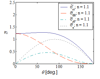
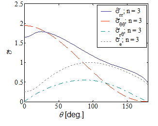
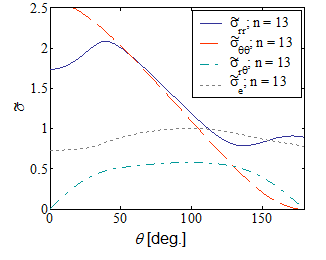
Let us examine the non-dimensional stress field around the crack tip. Picture VIII.3 to Picture VIII.5 show all the components of the non-dimensional stress field for different values of the hardening exponent $n$. It can be observed that the higher the hardening $n$, the larger is the variation in the stress components.
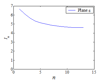
Now, let us remember that the near-tip stress field and strain field were expressed in terms of the $\frac{J E}{r\alpha\left(\sigma_p^0\right)^2I_n}$ in which $I_n$ has still to be determined, with
\begin{equation} I_n = \int_{-\pi}^{\pi} \tilde{h} \left(\theta,\,n\right) d\theta\,.\label{eq:Jint_In_2} \end{equation}
As a recall, the function $\tilde{h} \left(\theta,\,n\right)$, follows from the expression of the $J$-integral
\begin{equation}\label{eq:Jint_rew_2} J=\lim_{r\rightarrow 0} \int_{-\pi}^{\pi} \left(U \uV{n}_x - \defu_{,x}\cdot \cauchy\cdot \uV{n}\right) r d\theta = \frac{\alpha\left(\sigma_p^0\right)^2}{E} k_n^{n+1} \int_{-\pi}^{\pi} \tilde{h} \left(\theta,\,n\right) d\theta \,, \end{equation}
with the the near-tip stress field and the near-tip strain field (\ref{eq:J_stressstrain}). Since the displacement field is the strain field (\ref{eq:J_stressstrain}) integral, one can express it as
\begin{equation} \defu\left(r,\theta\right) \simeq \frac{\alpha\sigma_p^0}{E}k_n^nr^{\frac{1}{n+1}}\tilde{\defu}\,,\label{eq:J_u} \end{equation}
where the components vector $\tilde{\defu}$ is obtained by combining Eq. (\ref{eq:uStreamPolar}), Eq. (\ref{eq:StreamPhi}), and Eq. (\ref{eq:ftilde}) following
\begin{equation} \begin{cases} \tilde{\defu}_r\left(\theta\right) = -\tilde{g}'\,,\\ \tilde{\defu}_{\theta}\left(\theta\right) =\frac{n+2}{n+1}\tilde{g} \,. \end{cases}\label{eq:J_utilde} \end{equation}
Using the relation $\partial_x=\cos \theta \partial_r - \frac{\sin \theta}{r}\partial_\theta$, $\defu_{,x}$ is obtained from (\ref{eq:J_u}) as
\begin{equation} \defu_{,x} \left(r,\theta\right) \simeq \frac{\alpha\sigma_p^0}{E}k_n^nr^{\frac{-n}{n+1}}\left[\frac{\cos \theta}{n+1}\tilde{\defu}-\sin\theta \tilde{\defu}' \right]\,.\label{eq:J_upx} \end{equation}
The internal potential term has already been calculated as
\begin{equation} U =\frac{n\alpha\left(\sigma_p^0\right)^2}{E\left(n+1\right)} \frac{1}{r} k_n^{n+1}\sqrt{\frac{3}{2}\tilde{\uT{s}}:\tilde{\uT{s}} }^{n+1} \,. \end{equation}
Finally, since the normal component along $x$ reads $\uV{n}_x=\cos{\theta}$, and since the normal vector in polar coordinates reads $\uV{n}_r=1$, $\uV{n}_\theta=0$, the term $\tilde{h} \left(\theta,\,n\right)$ is deduced from (\ref{eq:Jint_rew_2}) using (\ref{eq:J_stressstrain}) as
\begin{equation}\label{eq:htilde}\begin{array}{ll} \tilde{h} \left(\theta,\,n\right) =& \frac{n}{\left(n+1\right)} \sqrt{\frac{3}{2}\tilde{\uT{s}}:\tilde{\uT{s}} }^{n+1} \cos\theta -\\ &\left[\frac{\cos \theta}{n+1}\tilde{\defu}-\sin\theta \tilde{\defu}' \right]\cdot \tilde{\cauchy}\cdot \uV{n} \,.\end{array} \end{equation}
The term $I_n$ (\ref{eq:Jint_In_2}) then follows from a simple integration and is illustrated in Picture VIII.6 for mode I and plane-$\varepsilon$ state.
Results for a semi-infinite crack in plane-$\varepsilon$ state
We have now fully defined the near-tip stress field and strain field in terms of the $J$-integral following
\begin{equation}\label{eq:stressField} \cauchy=\sigma_p^0\left(\frac{J E}{r\alpha\left(\sigma_p^0\right)^2I_n}\right)^{\frac{1}{n+1}}\tilde{\cauchy}\left(\theta,\,n\right)\,, \end{equation}
\begin{equation}\label{eq:strainField} \strain=\frac{\sigma_p^0\alpha}{E}\left(\frac{J E}{r\alpha\left(\sigma_p^0\right)^2I_n}\right)^{\frac{n}{n+1}} \tilde{\strain}\left(\theta,\,n\right)\,, \end{equation}
as well as the near-tip displacement field (\ref{eq:J_u}), which can be rewritten, using the expression of $k_n=\left(\frac{J E}{\alpha\left(\sigma_p^0\right)^2I_n}\right)^{\frac{1}{n+1}}$, as
\begin{equation} \defu\left(r,\theta\right) \simeq \frac{\alpha\sigma_p^0}{E}\left(\frac{J E}{\alpha\left(\sigma_p^0\right)^2I_n}\right)^{\frac{n}{n+1}} r^{\frac{1}{n+1}}\tilde{\defu}\,.\label{eq:uField} \end{equation}
In other words, once the $J$-integral has been evaluated, for example using a numerical method, the near-tip fields are known, and we can exploit their expressions to analyze the crack loading.
Process zone shape
Of particular interests are the shape and size of the process zone. For an elasto-plastic material, the process zone is defined as the zone in which plastic flow occurs. With our non-linear uncompressible material, the flow formally develops everywhere, but we can define a process zone in which $\sigma_e > \sigma_p^0$, whose boundary corresponds to $\sigma_e=\sigma_p^0$. This boundary is directly obtained using (\ref{eq:stressField}) as
\begin{equation}\label{eq:elasticPlastic_b} 1=\frac{\sigma_e}{\sigma_p^0} =\left(\frac{JE}{\alpha \left(\sigma_p^0\right)^2}\right)^{\frac{1}{n+1}} r^{-\frac{1}{n+1}} \tilde{\sigma}_e I_n^{-\frac{1}{n+1}} \, \text{.} \end{equation}
Let us introduce a non-dimensional radius $\tilde{r}$ given by
\begin{equation}\label{eq:nonDim_r} \tilde{r} = \frac{r \alpha \left(\sigma_p^0\right)^2 }{JE}\,, \end{equation}
so that the process zone boundary (\ref{eq:elasticPlastic_b}) can be rearranged as
\begin{equation} \tilde{r}\left(\theta,\,n\right) = \frac{\left(\tilde{\sigma}_e\left(\theta,\,n\right)\right)^{n+1}}{I_n} \, \text{.} \label{eq:processZone}\end{equation}
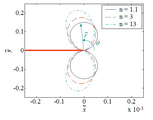
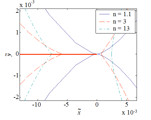
The process zone shape is depicted in Picture VIII.7 for varying hardening exponents and a zoom at the crack tip is provided in Picture VIII.8. For plane-$\varepsilon$ state, the process zone appears to have two round shapes above and below the crack tip for a low hardening exponent, and to exhibit a "propeller-like" shape with increasing $n$. Note that as it can be seen in Picture VIII.8, the process zone develop ahead of the crack tip and on the crack lips, in particular for increasing values of $n$.
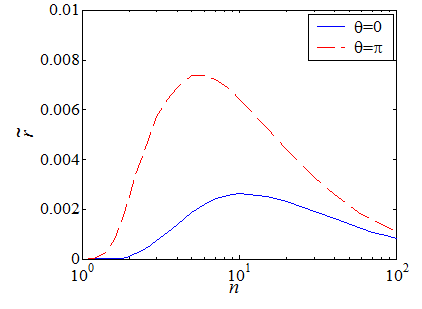
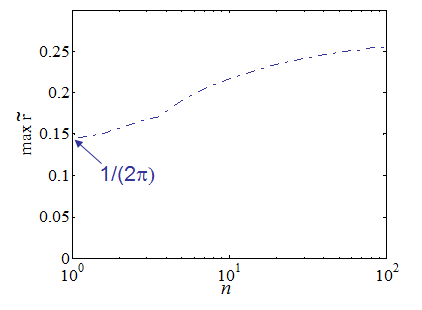
Besides the process zone shape, its size is also of interest. One can readily evaluate the size of the process zone in terms of $\tilde{r}$ ahead ($\theta=0$) and behind the crack tip ($\theta=\pi$) as shown in Picture VIII.9. However, the actual maximum value of $\tilde{r}$ is somewhere in between of $0 \leq \theta \leq \pi$ and is depicted as a function of the hardening exponent in Picture VIII.10. In particular, for $n\rightarrow 1$, linear-like behavior, the maximum radius is $\tilde{r}\rightarrow \frac{1}{2\pi}$.
Finally, note that under the SSY assumption one has $JE = K_I^2\left(1-\nu^2\right)$ under plane-$\varepsilon$ assumption, with $\nu=0.5$ for the considered uncompressible material. Therefore Eq. (\ref{eq:nonDim_r}) implies that the process zone size scales as
\begin{equation} r \propto \left(\frac{K_I}{\sigma_p^0}\right)^2\,. \end{equation}
Stress field at crack tip
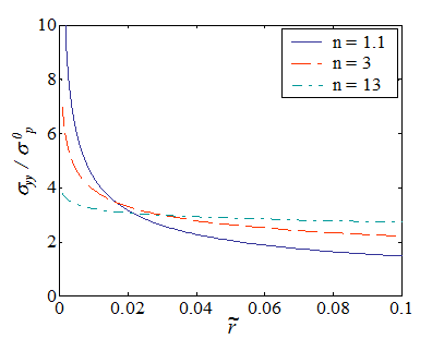
In order to assess the crack Mode I loading, the hoop stress is evaluated just ahead of crack tip $\theta=0$. Combining Eq. (\ref{eq:stressField}) and Eq. (\ref{eq:nonDim_r}), the hoop stress head of the crack lips reads
\begin{equation} \cauchy_{yy}\left(\theta=0\right) = \cauchy_p^0 \left(\frac{1}{\tilde{r} I_n}\right)^{\frac{1}{n+1}}\tilde{\cauchy}_{\theta\theta}\left(\theta=0,\,n\right) \, \text{.} \end{equation}
The stress field normalized over the yield stress is depicted in Picture VIII.11. As it can be seen, the HRR theory does not remove the stress singularity, except in the case $n\rightarrow\infty$. Since the abscissa is $\tilde{r} = \frac{r \alpha \left(\sigma_p^0\right)^2 }{JE}$, it appears that $J$ is a measure of the "intensity of the singularity" at crack tip (except in the case $n \rightarrow \infty$).
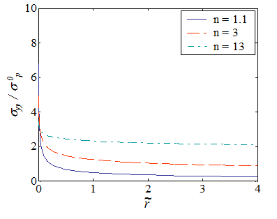
If we analyze the stress field further ahead from the crack tip, see Picture VIII.12, it appears that the HRR solution predicts a vanishing stress field. Indeed in the development of the method we have kept only the dominant term near crack tip. The HRR solution (\ref{eq:stressField}-\ref{eq:uField}) is thus an asymptotic solution as well.
Crack tip opening displacement (CTOD)
Besides the $J$-integral, a way to characterize the crack loading is to measure or evaluate its opening. The displacement field of the upper crack lip is given from (\ref{eq:uField}) by
\begin{equation}\label{eq:dispField_HRR} \defu\left(r,\,\pi\right) = \frac{\alpha \sigma_p^0}{E}\left(\frac{JE}{\alpha \left(\sigma_p^0\right)^2 I_n}\right)^{\frac{n}{n+1}} r^{\frac{1}{n+1}} \tilde{\defu}\left(\pi,\,n\right) \, \text{.} \end{equation}
Introducing the non-dimensional radius (\ref{eq:nonDim_r}) into (\ref{eq:dispField_HRR}), the displacement field becomes
\begin{equation} \defu\left(\tilde{r},\,\pi\right) = \frac{\alpha \sigma_p^0}{E} \frac{JE}{\alpha \left(\sigma_p^0\right)^2} \tilde{r}^{\frac{1}{n+1}} \frac{\tilde{\defu}\left(\pi,\,n\right)}{I_n^{\frac{n}{n+1}}} \, \text{.} \end{equation}
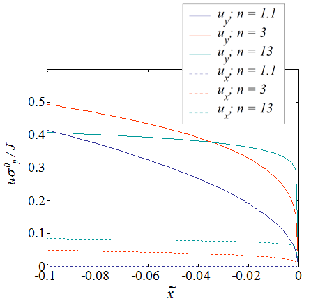
The components of the crack displacement field of the upper lip ($\theta=\pi$) in terms of the non-dimensional value $\tilde{x}=-\tilde{r}$ are illustrated on Picture VIII.13, where it is seen that a point of lip is experiencing a vertical displacement, corresponding to an opening, but also an horizontal displacement toward the crack tip, following the schematics in Picture VIII.14. Let us define the crack opening displacement (COD) $\delta$ shown in Picture VIII.14 as the distance between the crack lips, which is by symmetry of the mode I loading
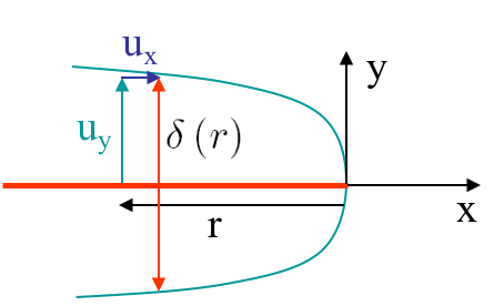
\begin{equation} \delta\left(r\right) = 2\defu_y\left(r,\,\pi\right) \, \text{.} \end{equation}
The COD is always positive along $x<0$ and is equal to zero at crack tip, see Picture VIII.13. This is a difference to the Dugdale's model, for which a positive crack opening tip displacement (CTOD) was found at $x=0$. Therefore, since the COD $\delta\left(r\right)$ depends on $x$ and vanishes at crack tip for the HRR theory, can we define a representative crack tip opening displacement (CTOD)? The CTOD $\delta_t$ is defined as $\delta\left(r\right)$ such that a 90$^{\circ}$ angle is intercepted at the crack tip, see Picture VIII.15. Let us denote radius $r$, which satisfies this criterion, by $r^{*}$. Remembering that the upper lip experiences both a horizontal and a vertical displacements (so the material point $x$ position is not the one at which the vertical displacement is measured), one has
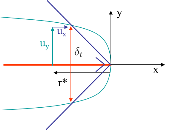
\begin{equation}\label{eq:CTOD_radius} r^*-\defu_x\left(r^*,\,\pi\right) = \defu_y\left(r^*,\,\pi\right)=\frac{\delta_t}{2} \, \text{.} \end{equation}
Inserting (\ref{eq:dispField_HRR}) into (\ref{eq:CTOD_radius}) yields $r^{*}$
\begin{equation} r^*= \left(\frac{\alpha \sigma_p^0}{E}\right)^{\frac{1}{n}}\left(\frac{J}{\sigma_p^0 I_n}\right) \left[\tilde{\defu}_x\left(\pi,\,n\right)+ \tilde{\defu}_y\left(\pi,\,n\right)\right]^{\frac{n+1}{n}}\,, \end{equation}
or again $r^{*\frac{1}{n+1}}$ as
\begin{equation} {r^*}^\frac{1}{n+1}= \left(\frac{\alpha \sigma_p^0}{E}\right)^{\frac{1}{n\left(n+1\right)}}\left(\frac{J}{\sigma_p^0 I_n}\right)^\frac{1}{n+1} \left[\tilde{\defu}_x\left(\pi,\,n\right)+ \tilde{\defu}_y\left(\pi,\,n\right)\right]^{\frac{1}{n}} \, \text{.} \end{equation}
Therefore, inserting this last result in (\ref{eq:dispField_HRR}) allows expressing the CDOT (\ref{eq:CTOD_radius}) as
\begin{equation} \delta_t = 2\defu_y\left(r^*,\,\pi\right)= 2\left(\frac{\alpha \sigma_p^0}{E}\right)^{\frac{1}{n}}\left(\frac{J}{\sigma_p^0 I_n}\right) \left[\tilde{\defu}_x\left(\pi,\,n\right)+ \tilde{\defu}_y\left(\pi,\,n\right)\right]^{\frac{1}{n}}\tilde{\defu}_y\left(\pi,\,n\right) \, \text{.} \label{eq:ctodtmp}\end{equation}
The expression of the CTOD (\ref{eq:ctodtmp}) not only depends on the $J$-integral, but also on the elastic strain $\frac{\alpha \sigma_p^0}{E}$, and of course of the function $\tilde{\defu}\left(\pi,\,n\right)$. Therefore, in order to simply the expression, we introduce the following variable $d_n$
\begin{equation} d_n= 2\left(\frac{\alpha \sigma_p^0}{E}\right)^{\frac{1}{n}}\left(\frac{1}{I_n}\right) \left[\tilde{\defu}_x\left(\pi,\,n\right)+ \tilde{\defu}_y\left(\pi,\,n\right)\right]^{\frac{1}{n}}\tilde{\defu}_y\left(\pi,\,n\right) \, \text{,} \end{equation}
and the CTOD can be expressed in the compact form of
\begin{equation} \delta_t = d_n\frac{J}{\sigma_p^0} \, \text{.} \label{eq:CTODHRR}\end{equation}
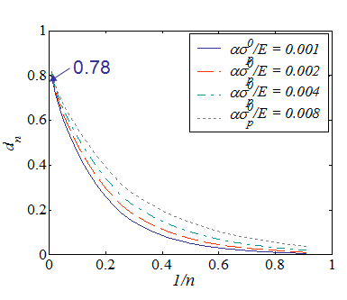
Contrarily to the other analyzed features of the HRR theory, the value of $d_n$ depends on $n$ but also on the elastic strain of the considered material $\frac{\alpha\sigma^0_p}{E}$. Its evolution with the hardening exponent is computed for different ratios of $\frac{\alpha\sigma^0_p}{E}$ in Picture VIII.16. The value of $d_n$ is higher when $n\rightarrow \infty$ and has a low dependency on $\frac{\alpha\sigma^0_p}{E}$. Therefore, it can be concluded that, for a given material, $J$ is uniquely related to the CTOD $\delta_t$ and this last one can be used as a crack initiation criterion such as $\delta_t \geq \delta_C$, where $\delta_C=d_n\frac{J_C}{\sigma_p^0}$ is the critical crack opening.
Summary for a semi-infinite crack in plane-$\varepsilon$ state
Lastly, before going to the next sections, the most important points so far should be summarized.
To develop the HRR near-tip fields such as displacement, strain and stress fields, the following assumptions were made:
- Small deformations;
- There is no unloading and loading is proportional in all the directions (so the theory is formally valid only for crack initiation and not for crack propagation);
- Elastic strains are assimilated to plastic strain (so the material is assumed to be incompressible) ;
- J2-plasticity with power law description;
- Semi-infinite crack.
We have then solved the equations of the HRR theory for semi-infinite mode I crack loading in plane-$\varepsilon$ state, for which the following can be stated:
-
The asymptotic stress field follows
\begin{equation}
\cauchy=\sigma_p^0\left(\frac{J E}{r\alpha\left(\sigma_p^0\right)^2I_n}\right)^{\frac{1}{n+1}}\tilde{\cauchy}\left(\theta,\,n\right) \, \text{.}
\end{equation}
- The $J$-integral plays the role of an equivalent "plastic strain intensity factor".
- The stress field evolves in a proportional way with $J$, so the theory is applicable to incremental plasticity as long as $J$ increases.
- We were able to describe the process zone by \begin{equation} \tilde{r}\left(\theta,\,n\right) = \frac{\left( \tilde{\sigma}_e\left(\theta,\,n\right)\right)^{n+1}}{I_n}\,, \end{equation} with $\tilde{r} = \frac{r \alpha \left(\sigma_p^0\right)^2 }{JE}$. Therefore, if we assume SSY, the process zone would scale by $ r \propto \left(1-\nu^2\right) \left(\frac{K_I}{\sigma_p^0}\right)^2$.
- A new definition for the CTOD was made with $\delta_t = d_n\frac{J}{\sigma_p^0}$, which is also a function of $J$.
- We did not assume SSY !!!
Two questions remains which will be the topic in the next sections. What does happen for other configurations? What is the range of validity of the HRR theory?
![]()