
Energetic Approach > J-Integral
As seen in the previous pages, the crack closure integral has some limitations: It can only be "easily" computed for linear and elastic materials, and is useful for cracks growing straight ahead only. The following introduces a more general energy-related concept called the J-Integral.
The J-integral concept
Homogeneous bodies
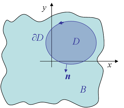
In 1968, Rice suggested to compute the energy that flows toward the crack tip. To do so he considered a homogeneous un-cracked body $B$ with the following conditions:
- $D$ is a sub-volume of boundary $\partial D$;
- The stress tensor derives from a potential $U$;
- On the boundary $\partial D$, traction forces $\mathbf{T}$ are defined as $\mathbf{\sigma} \cdot \mathbf{n}$;
- The problem is static, so $\nabla \cdot \mathbf{\sigma} = 0$.
Using these notations the J-integral is a vector defined as:
\begin{equation} \mathbf{J} = \int_{\partial D} \left[U\left(\mathbf{\nabla}\mathbf{u}\right) \mathbf{n} - \left(\mathbf{\nabla}\mathbf{u}\right)^T \mathbf{T}\right]dA,\label{eq:Jintegral} \end{equation}
or, in the indicial form:
\begin{equation}
\mathbf{J}_i = \int_{\partial D} \left[U\left(\mathbf{\varepsilon}\right) \mathbf{n}_i -
\mathbf{\nabla}_i \mathbf{u}_k \mathbf{\sigma}_{km} \mathbf{n}_m\right] dA.\label{eq:JintegralIndices}
\end{equation}
As $\mathbf{\sigma}^T=\mathbf{\sigma}$ and $\nabla \cdot \mathbf{\sigma} = 0$, applying the Gauss theorem on this last expression leads to
\begin{eqnarray} \mathbf{J}_i &=& \int_{D} \left[\underbrace{\frac{\partial U}{\partial \mathbf{\varepsilon}_{km}}}_{\mathbf{\sigma}_{km}}\frac{\mathbf{u}_{k,mi}+\mathbf{u}_{m,ki}}{2} - \mathbf{\sigma}_{km}\mathbf{u}_{k,im}-\underbrace{\mathbf{\sigma}_{km,m}}_{=0}\mathbf{u}_{k,i} \right] dD=\mathbf{\sigma}_{km}\mathbf{u}_{k,mi}- \mathbf{\sigma}_{km}\mathbf{u}_{k,im}= 0. \label{eq:Jhomog}\end{eqnarray}
This relation means that the energy flowing through a closed surface in an homogeneous medium is equal to zero. But what happens if the body is heterogeneous or cracked?
Heterogeneous bodies
For heterogeneous bodies the internal material potential $U(\mathbf{\nabla} \mathbf{u},\, \mathbf{X})$ depends on the position $\mathbf{X}$, so when applying the Gauss theorem we should consider that
\begin{equation} \frac{D U\left(\mathbf{\nabla}\mathbf{u},\mathbf{X}\right)}{D\mathbf{X}_i} = \frac{\partial U}{\partial \mathbf{\varepsilon}}:\mathbf{\varepsilon}_{,i} +\frac{\partial U}{\partial \mathbf{X}_i}. \end{equation}
As a result $\mathbf{J} \neq 0$ even for un-cracked bodies as the second term remains in (\ref{eq:Jhomog}).
Cracked homogeneous bodies (2D)
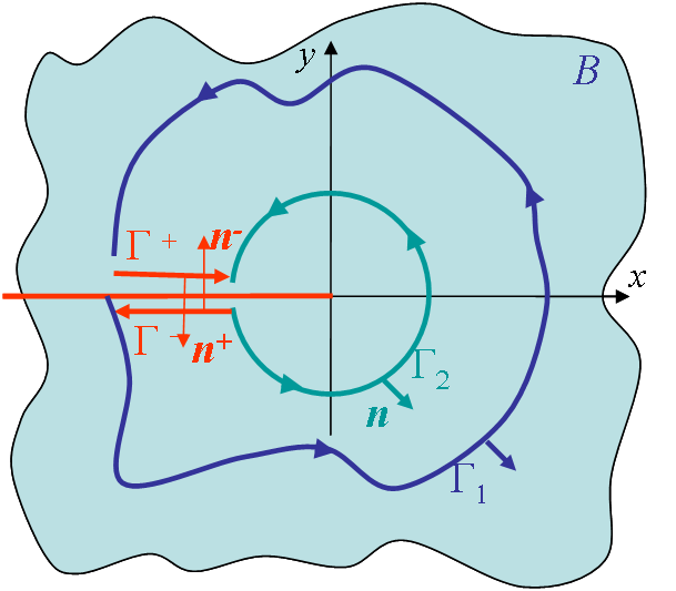
Let us now consider a cracked homogeneous material. We can still use (\ref{eq:Jhomog}) if the contour $\Gamma$ embeds a homogeneous part, meaning if it does not intercept the crack. Considering a crack parallel to the x-axis with the contour $\Gamma=\Gamma_1+\Gamma^++\Gamma^--\Gamma_2$ going around the crack, see Picture III.26, then (\ref{eq:Jhomog}) is satisfied and
\begin{equation} \mathbf{J}_x = \oint_\Gamma \left[U\left(\mathbf{\varepsilon}\right) \mathbf{n}_x - \mathbf{\mathbf{u}}_{,x} \cdot \mathbf{T}\right] dl = 0, \label{eq:JCrackedFull} \end{equation}
with $\oint_\Gamma = \int_{\Gamma_1} + \int_{\Gamma^+}+ \int_{\Gamma^-} - \int_{\Gamma_2}$. We can now analyze the contribution on the different curves. Along $\Gamma^+$ and $\Gamma^-$ we have
- $\mathbf{n}_x = 0$ and $\mathbf{n}_y \pm 1$;
- The crack is stress-free (no friction): $\mathbf{T}_\alpha = \mathbf{\sigma}_{\alpha y} \mathbf{n}_y = 0$;
- Hence $\int_{\Gamma^-} =\int_{\Gamma^+} = 0$.
So (\ref{eq:JCrackedFull}) simplifies into the so-called J-integral, which is the energy that flows toward the crack tip:
\begin{equation} J = \int_{\Gamma_1} \left[U\left(\mathbf{\varepsilon}\right) \mathbf{n}_x - \mathbf{\mathbf{u}}_{,x} \cdot \mathbf{T}\right] dl = \int_ {\Gamma_2} \left[U\left(\mathbf{\varepsilon}\right) \mathbf{n}_x - \mathbf{\mathbf{u}}_{,x} \cdot \mathbf{T}\right] dl.\label{eq:J} \end{equation}
As it can be deduced from (\ref{eq:J}), this integral
- Is path independent (as long as the contour embeds the crack tip);
- Does not request linearity of the material (only the existence of an internal potential has been assumed);
- Does not depend on subsequent crack growth direction.
This concept is thus particularly general and is widely used in analytical and numerical analyzes, as it will be shown later.
Particular cases and the J-integral
Although the concept is general as long as an internal potential exists, the J-Integral can be specialized and in particular can be related to the concepts of energy release rate and of SIFs studied before.
For cracks growing straight ahead
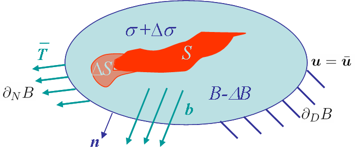
Heading back to the crack closure integral, we have found the following potential energy variation for a growing cavity, see Picture III.27:
\begin{eqnarray} \Delta \Pi_T &=& \int_{B-\Delta B} U\left(\mathbf{\nabla}\mathbf{u}+\mathbf{\nabla}\Delta\mathbf{u}\right)-U\left(\mathbf{\nabla}\mathbf{u}\right) dB-\nonumber\\&&\int_{\Delta B} U\left(\mathbf{\nabla}\mathbf{u}\right) dB - \int_{\partial_N B} \bar{\mathbf{T}} \cdot\Delta\mathbf{u}d\partial B.\label{eq:DpiCCI1} \end{eqnarray}
The energy release rate for a crack (no change of volume) can thus be evaluated as
\begin{eqnarray}
G = \lim_{\Delta a \rightarrow 0} - \frac{\Delta \Pi_T}{ t \Delta a} =
\lim_{\Delta a \rightarrow 0} \frac{1}{\Delta a}\left\{ \int_{B}
U\left(\mathbf{\nabla}\mathbf{u}\right) -U\left(\mathbf{\nabla}\mathbf{u}+\mathbf{\nabla}\Delta\mathbf{u}\right) d B + \int_{\partial_N B} \bar{\mathbf{T}} \cdot \Delta\mathbf{u} d \partial B\right\}.\label{eq:JToG1}
\end{eqnarray}
As the crack is stress-free, as $\Delta \mathbf{u}=0$ on $\partial_DB$, and as $\Delta\mathbf{\sigma}=0$ on $\partial_N B$, the last term of this equation can be simplified into
\begin{equation} \int_{\partial_N B}\bar{\mathbf{T}} \cdot \Delta \mathbf{u} d \partial B = \int_{\partial_N B+\partial_D B + S+\Delta S} \Delta \mathbf{u}\cdot \left(\mathbf{\sigma}+\Delta\mathbf{\sigma}\right)\cdot \mathbf{n} d \partial B = \int_{B} \mathbf{\nabla}\cdot\left( \Delta \mathbf{u}\cdot \left(\mathbf{\sigma}+\Delta\mathbf{\sigma}\right)\right) d B.\label{eq:JToG2}, \end{equation}
or, as $\mathbf{\nabla}\cdot\mathbf{\sigma}=\mathbf{\nabla}\cdot\left(\mathbf{\sigma}+\Delta\mathbf{\sigma}\right)=0$, into
\begin{equation} \int_{\partial_N B}\bar{\mathbf{T}} \cdot \Delta \mathbf{u} d \partial B = \int_{B} \left(\mathbf{\sigma}+\Delta\mathbf{\sigma}\right):\left(\mathbf{\nabla} \Delta \mathbf{u}\right) d B\label{eq:JToG3}. \end{equation}
Using this last result in (\ref{eq:JToG1}) yields
\begin{equation}
G = \lim_{\Delta a \rightarrow 0} \frac{1}{\Delta a}\left\{ \int_{B}
U\left(\mathbf{\varepsilon}\right) - U\left(\mathbf{\varepsilon}+\Delta\mathbf{\varepsilon}\right) +
\left(\mathbf{\sigma}+\Delta\mathbf{\sigma}\right):\Delta\mathbf{\varepsilon} d B\right\}.\label{eq:JToG4}
\end{equation}
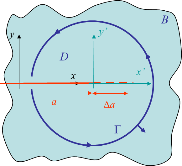
Assuming the crack grows straight ahead we can consider the following change of variables, see Picture III.28,
\begin{equation} \begin{cases} x' = x- a\\ y' = y \end{cases} \rightarrow \begin{cases}f(x',y',a) = f(x-a,y,a) \\ \frac{d f}{d a} = - \partial_{x'} f +\partial_a f\end{cases}. \label{eq:JToGCV}\end{equation}
The energy release rate (\ref{eq:JToG4}) involves the whole body $B$. However as $\Delta a\rightarrow 0$, the non-vanishing contributions are around the crack tip. So we can limit the integral to a fixed region $D$ of boundary $\Gamma$, see Picture III.28, and this equation becomes
\begin{eqnarray} G = \lim_{\Delta a \rightarrow 0} \frac{1}{\Delta a}&&\left\{ \int_{D} U\left(\mathbf{\varepsilon}\right) - U\left(\mathbf{\varepsilon}+\Delta\mathbf{\varepsilon}\right) +\right.\nonumber\\&&\left.\left(\mathbf{\sigma}+\Delta\mathbf{\sigma}\right):\Delta\mathbf{\varepsilon} d D\right\}.\label{eq:JToG5} \end{eqnarray}
We can integrate by parts and apply the Gauss theorem on the last term of (\ref{eq:JToG5}), and as $\mathbf{\nabla}\cdot\left(\mathbf{\sigma}+\Delta\mathbf{\sigma}\right)=0$, it yields
\begin{equation} \int_D \left(\mathbf{\sigma}+\Delta \mathbf{\sigma}\right): \Delta \mathbf{\varepsilon} dD = \int_\Gamma \Delta \mathbf{u}\cdot\left(\mathbf{\sigma}+\Delta \mathbf{\sigma}\right)\cdot\mathbf{n} dl ,\label{eq:JToG6}\end{equation}
or
\begin{equation}\lim_{\Delta a\rightarrow 0}\frac{1}{\Delta a} \int_D \left(\mathbf{\sigma}+\Delta \mathbf{\sigma}\right): \Delta \mathbf{\varepsilon} dD =\lim_{\Delta a\rightarrow 0}\frac{1}{\Delta a} \int_\Gamma \Delta \mathbf{u}\cdot\left(\mathbf{\sigma}+\Delta \mathbf{\sigma}\right)\cdot\mathbf{n} dl .\label{eq:JToG8}\end{equation}
Considering the change of variables (\ref{eq:JToGCV}), this last equation reads
\begin{equation}\lim_{\Delta a\rightarrow 0}\frac{1}{\Delta a} \int_D \left(\mathbf{\sigma}+\Delta \mathbf{\sigma}\right): \Delta \mathbf{\varepsilon} dD =\int_\Gamma \frac{d
\mathbf{u}}{d a} \cdot \mathbf{T} dl = \int_\Gamma \left( - \partial_{x'}
\mathbf{u} +\partial_a \mathbf{u} \right) \cdot \mathbf{T} dl. \label{eq:JToG9}\end{equation}
One more time using $\mathbf{\nabla}\cdot\mathbf{\sigma}=\mathbf{\nabla}\cdot\partial_{\mathbf{\varepsilon}}U=0$ we have
\begin{equation} \int_\Gamma \partial_a \mathbf{u} \cdot \mathbf{T} dl = \int_\Gamma \partial_a\mathbf{u} \cdot \partial_{\mathbf{\varepsilon}} U \cdot \mathbf{n} dl = \int_D
\partial_a\mathbf{\varepsilon} : \partial_{\mathbf{\varepsilon}} U d D = \int_D
\partial_a U d D,\label{eq:JToG10} \end{equation}
and (\ref{eq:JToG9}) reads
\begin{equation}\lim_{\Delta a\rightarrow 0}\frac{1}{\Delta a} \int_D \left(\mathbf{\sigma}+\Delta \mathbf{\sigma}\right): \Delta \mathbf{\varepsilon} dD = - \int_\Gamma \partial_{x'}
\mathbf{u} \cdot \mathbf{T} dl + \int_D \partial_a U d D. \label{eq:JToG11}\end{equation}
We can now consider the first term of (\ref{eq:JToG5}). The domain $D$ is fixed to the initial crack tip, but we can define a domain $D^\star$ moving with the crack tip such that $D=D^\star+\Delta D_L-\Delta D_R$, see Picture III.29. The first term of (\ref{eq:JToG5}) reads
\begin{eqnarray} \lim_{\Delta a \rightarrow 0} \frac{1}{\Delta a}\int_{D} U\left(\mathbf{\varepsilon}\right) - U\left(\mathbf{\varepsilon}+\Delta\mathbf{\varepsilon}\right) d D =\quad\quad\quad\quad\nonumber\\
\lim_{\Delta a \rightarrow 0} \frac{1}{\Delta a}\left\{ \int_{D}
U\left(\mathbf{\varepsilon}\left(a\right)\right) dD -\right.\quad\quad\nonumber\\
\left. \int_{D*+\Delta D_L -
\Delta D_R} U\left(\mathbf{\varepsilon}\left(a+\Delta a\right)\right) d D\right\}.\label{eq:JToG12}
\end{eqnarray}
As $D^\star \rightarrow D$ for infinitesimal crack growth, this relation becomes (formally, one should use derivatives & limits of integrals with non-constant intervals)
\begin{eqnarray} \lim_{\Delta a \rightarrow 0} \frac{1}{\Delta a}\int_{D} U\left(\mathbf{\varepsilon}\right) - U\left(\mathbf{\varepsilon}+\Delta\mathbf{\varepsilon}\right) d D &=&
\lim_{\Delta a \rightarrow 0} \left\{ \int_{D} \frac{U\left(\mathbf{\varepsilon}\left(a\right)\right)-U\left(\mathbf{\varepsilon}\left(a+\Delta a\right)\right) }{\Delta a} dD -\right.\nonumber\\
&&\left. \frac{1}{\Delta a} \int_{\Delta D_L - \Delta D_R} U\left(\mathbf{\varepsilon}\left(a+\Delta a\right)\right) d D\right\}
.\label{eq:JToG13}\end{eqnarray}
These integrals can be successively computed:
- As we have an homogeneous material, one has $\partial_{x'}U=0$ and \begin{equation} \lim_{\Delta a \rightarrow 0} \int_{D} \frac{U\left(\mathbf{\varepsilon}\left(a\right)\right)-U\left(\mathbf{\varepsilon}\left(a+\Delta a\right)\right) }{\Delta a} dD = -\int_{D} \partial_a U dD.\label{eq:JtoGtmp1} \end{equation}
-
Considering the left increment $\Delta D_L$ and the open curve $\Gamma_L$, see Picture III.30, for an infinitesimal crack advance we have \begin{equation}
\int_{\Delta D_L} U d D = \int_{-\Gamma_L} U \mathbf{n}_x \Delta a dl, \end{equation} so that
\begin{equation} \lim_{\Delta a \rightarrow 0}\frac{1}{\Delta a} \int_{\Delta D_L} U\left(\mathbf{\varepsilon}\left(a+\Delta a\right)\right) d D = -\int_{ \Gamma_L} U\left(\mathbf{\varepsilon}\left(a\right)\right)\mathbf{n}_x d l\label{eq:JtoGtmp2}. \end{equation}
-
Considering the right increment $\Delta D_R$ and the open curve $\Gamma_R^\star$, see Picture III.31, for infinitesimal crack advance we have \begin{equation}
\int_{\Delta D_R} U d D = \int_{\Gamma_R} U \mathbf{n}_x \Delta a dl, \end{equation} so that
\begin{equation} \lim_{\Delta a \rightarrow 0}\frac{1}{\Delta a} \int_{\Delta D_R} U\left(\mathbf{\varepsilon}\left(a+\Delta a\right)\right) d D = \int_{ \Gamma_R^\star} U\left(\mathbf{\varepsilon}\left(a\right)\right)\mathbf{n}_x d l\label{eq:JtoGtmp3}. \end{equation}
Combining (\ref{eq:JtoGtmp1}-\ref{eq:JtoGtmp3}), and as $\Gamma_L + \Gamma_R^\star\rightarrow $\Gamma$, the relation (\ref{eq:JToG13}) becomes
\begin{equation} \lim_{\Delta a \rightarrow 0} \frac{1}{\Delta a}\int_{D} U\left(\mathbf{\varepsilon}\right) - U\left(\mathbf{\varepsilon}+\Delta\mathbf{\varepsilon}\right) d D=-\int_{D} \partial_a U dD +\int_{ \Gamma} U\left(\mathbf{\varepsilon}\left(a\right)\right)\mathbf{n}_x d l .\label{eq:JToG14} \end{equation}
If the crack grows straight ahead, for $\Delta a \rightarrow 0$, we have found (\ref{eq:JToG11}) and (\ref{eq:JToG14}) which are summarized as
\begin{equation} \begin{cases}
\lim_{\Delta a \rightarrow 0} \frac{1}{\Delta a}\int_{D}
U\left(\mathbf{\varepsilon}\right) - \left(\mathbf{\varepsilon}+\Delta\mathbf{\varepsilon}\right) d D =
-\int_{D} \partial_a U dD +\int_{ \Gamma}
U\left(\mathbf{\varepsilon}\left(a\right)\right)\mathbf{n}_x dl \\
\lim_{\Delta a\rightarrow 0}\frac{1}{\Delta a} \int_D
\left(\mathbf{\sigma}+\Delta \mathbf{\sigma}\right): \Delta \mathbf{\varepsilon} dD = - \int_\Gamma \partial_{x'}
\mathbf{u} \cdot \mathbf{T} dl + \int_D
\partial_a U d D \end{cases},
\end{equation}
so that (\ref{eq:JToG5}) finally reads
\begin{equation}
G = \int_{ \Gamma}
U\left(\mathbf{\varepsilon}\left(a\right)\right)\mathbf{n}_x d l- \int_\Gamma \partial_{x}
\mathbf{u} \cdot \mathbf{T} dl = J.
\end{equation}
So, if the material is defined by an internal potential and if the crack grows straight ahead, $G=J$.
Linear Elasticity
Let us now consider the case of linear elastic materials. The general expression of $J$ reads
\begin{equation} J = \int_{\Gamma} \left[U\left(\mathbf{\varepsilon}\right) \mathbf{n}_x - \mathbf{u}_{,x} \cdot \mathbf{T}\right] dl, \label{eq:Jelast1}\end{equation}
and can be particularized for linear elasticity ($U=\frac{\mathbf{\sigma}\mathbf{\varepsilon}}{2}$) as
\begin{equation} J = \int_{\Gamma} \left[\frac{\mathbf{\sigma}_{ij}\mathbf{u}_{i,j}}{2}\delta_{xk} - \mathbf{u}_{i,x} \mathbf{\sigma}_{ik}\right]\mathbf{n}_k dl .\label{eq:Jelast2}\end{equation}
Let the contour $\Gamma$ be a circle as shown in Figure III.32. Thus as
\begin{equation} \begin{pmatrix} \partial_x \\ \partial_y \end{pmatrix} = \begin{pmatrix} \cos \theta & -\frac{\sin \theta}{r} \\ \sin \theta & \frac{\cos \theta}{r} \end{pmatrix} \begin{pmatrix} \partial_r \\ \partial_\theta \end{pmatrix},\label{eq:Jelast3} \end{equation}
the J-Integral (\ref{eq:Jelast2}) becomes
\begin{eqnarray}
J &=& \int_{-\pi}^{\pi} \frac{r\mathbf{\sigma}_{ix}\cos{\theta}u_{i,r}-\mathbf{\sigma}_{ix}\sin{\theta}u_{i,\theta}+
r \mathbf{\sigma}_{iy} \sin{\theta}u_{i,r} +
\mathbf{\sigma}_{iy}\cos{\theta}u_{i,\theta}}{2}\cos{\theta}
d\theta-\nonumber\\
&& \int_{-\pi}^{\pi}
\left[r\mathbf{\sigma}_{ix}\cos{\theta}u_{i,r}-\mathbf{\sigma}_{ix}\sin{\theta}u_{i,\theta}\right]\cos{\theta}
d\theta-\nonumber\\&& \int_{-\pi}^{\pi}
\left[r\mathbf{\sigma}_{iy}\cos{\theta}u_{i,r}-\mathbf{\sigma}_{iy}\sin{\theta}u_{i,\theta}\right]\sin{\theta}
d\theta \label{eq:Jelast4}.\end{eqnarray}
As J is path-independent we can take $r$ tending to 0 and can thus use the asymptotic solution
\begin{equation} \begin{cases} \mathbf{\sigma}^\text{mode i} = \frac{K_i}{\sqrt{2 \pi r}} \mathbf{f}^\text{mode i}(\theta) \\ \mathbf{u}^\text{mode i} = K_i \sqrt{\frac{r}{2 \pi}} \mathbf{g}^\text{mode i}(\theta) \end{cases}. \end{equation}
Superposing the fracture modes yields
\begin{equation} \begin{cases} \mathbf{u} = \sqrt{\frac{r}{2\pi}}\sum_{i=I}^{III} K_i \mathbf{g}^{\text{mode i}}\left(\theta\right) \\ \mathbf{\sigma} = \frac{1}{\sqrt{2\pi r}}\sum_{i=I}^{III} K_i \mathbf{f}^{\text{mode i}}\left(\theta\right) \end{cases}, \end{equation}
and after some manipulations the J-integral (\ref{eq:Jelast4}) becomes
\begin{equation} J = \frac{K^2_I}{E'}+\frac{K^2_{II}}{E'}+\frac{K^2_{III}}{2\mu}.\label{eq:Jelast5} \end{equation}
So, if the material is linear and elastic for any direction of the crack growth $J=\frac{K^2_I}{E'}+\frac{K^2_{II}}{E'}+\frac{K^2_{III}}{2\mu}$.