
\(\newcommand{\cauchy}{\boldsymbol{\sigma}}\) \(\newcommand{\strain}{\boldsymbol{\varepsilon}}\) \(\newcommand{\uV}{\boldsymbol}\) \(\newcommand{\uT}{\boldsymbol}\) \(\newcommand{\defu}{\boldsymbol{u}}\)
HRR theory > Outcomes of the HRR models
So far, we have derived the HRR asymptotic solution. At this point, we want to discuss the practical outcomes of the theory, and what we can actually learn from these models.
HRR solution can explain 3D effects
One of the advantages of the HRR solution is that it can explain 3D effects in crack propagation. Let us assume a specimen with an edge-crack. When applying the HRR theory, the solution is either
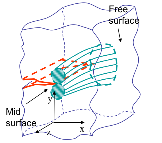
- Plane-$\sigma$-like near the free surfaces (where the material can actually expand laterally); or
- Plane-$\varepsilon$-like near the mid-plane of a specimen (where by symmetry the material does not expand laterally).
Both solutions are depicted in Picture VIII.30, where it can be seen that the shape of the process zone evolves from a "propeller-like" at mid-section to the more diffuse process zone at the specimen free faces.
Although the $J$-integral is formally not constant along the crack front through the thickness, it remains that
- There is a transition in the plastic zone shape and size;
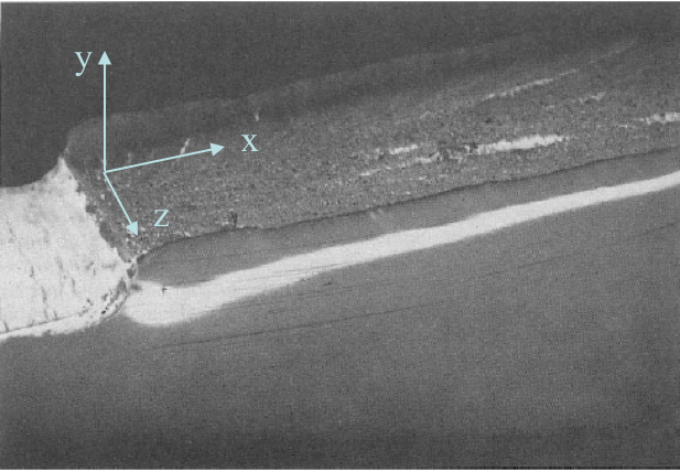
- This transition is responsible for the shear lips;
- Shear lips form at a 45$^{\circ}$ angle since $\sigma_{zz}=0$ so that the maximum shear stress is at 45$^{\circ}$ in the plane Oyz, see Picture VIII.31.
Assuming SSY, and performing a toughness test, the real value of $K$ changes along the crack front, so that the measured value of $K$ is an average one. As a results
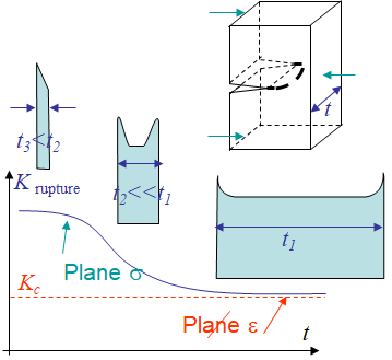
- The measured value of $K$ is more important for thin specimen, since the part of the specimen under plane-$\varepsilon$ state is relatively less important;
- For thick specimen, the process zone is mainly under plane-$\varepsilon$ state, although the free surfaces remain under plane-$\sigma$ state, and the measured $K$ stabilized to the so called plane-$\varepsilon$ critical $K$, the toughness, as indicated in Picture VIII.32, see also Lecture 2.
Nevertheless, there actually exist complex 3D effects:
- Under SSY assumption, even for a thin specimen, a plane-$\varepsilon$ state generally develops near the mid-plane.
- However, if the load increases (or the specimen thickness decreases), the plastic zone can become plane-$\sigma$-like near the mid-plane.
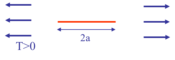
Rigorously, the effect of the specimen thickness results from triaxiality effect. Remember that under SSY assumption, the stress intensity factor characterizes the dominant term at crack tip, but at a larger distance, the other series terms are not negligible anymore, see Lecture 5. Effect of $T$-stress, see Picture VIII.33, should also be considered:
- Recall $T$-stress is the 0-order term obtained with the asymptotic solution, which is dominant at a distance $r_c$ from crack tip;
- In general, if the toughness test is such that $T<0$, the measured fracture $K$ will be larger than for $T>0$, independently of the thickness (see D.J. Smith, M.R. Ayatollahi and M.J. Pavier, Proc. R. Soc. A, 2006, vol. 462, pp 415-2437).
- For ASTM toughness tests, the thickness is large $t > 2.5 \left(\frac{K_C}{\sigma_p^0}\right)^2$ so that $T>0$.
Effective crack length for SSY
Another outcome of the HRR theory was the prediction of the process zone size. If the SSY assumption holds true, then
- $J$ can be expressed in terms of $K$;
- Then the plastic size can be written $r \propto \frac{JE}{\left(\sigma_p^0\right)^2} \propto \left(\frac{K_I}{\sigma_p^0}\right)^2$;
- However, there are dependencies on
- The parameters $n$ (plasticity) and $\nu$ (compressibility) and
- Whether it is plane-$\varepsilon$ or plane-$\sigma$ state.
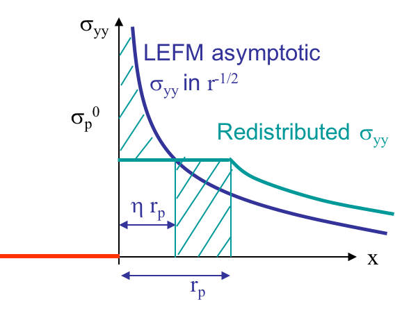
In the case of perfectly plastic materials $\left( n\rightarrow \infty \right)$, Rice has developed a model to predict the process zone size, based on a redistribution of the stress at crack tip, see Picture VIII.34. When assuming linear elasticity, the Mode I asymptotic solution predicts an infinite stress at crack tip, following
\begin{equation} \cauchy_{yy}\left(r,\theta=0\right) = \frac{K_I}{\sqrt{2\pi r}}\,. \label{eq:LEFM}\end{equation}
blue line, which is not physical. At crack tip the stress is limited by the yield stress $\sigma_p^0$. However, there should be a stress redistribution so that the total load remains constant, leading to the green line for which the process zone extend to a length $r_p$. The model is then solved in two steps:
- Evaluation of the intersection between the linear elastic solution with the yield stress at a fraction $\eta$ of the process zone. Using Eq. (\ref{eq:LEFM}) yields \begin{equation}\label{eq:rice_1} \sqrt{\eta r_p} = \frac{1}{\sqrt{2\pi}}\frac{K_I}{\sigma_p^0}\,. \end{equation}
- Equivalence between the total traction values of the LEFM solution (\ref{eq:LEFM}) and of the shifted green solution. Outside the plastic zone, the stress distribution is shifted, and the two hashed parts of Picture VIII.34 should have the same area: \begin{equation}\label{eq:rice_2} \sigma_p^0 \left(1-\eta\right)r_p = \int_0^{\eta r_p} \left(\cauchy_{yy}-\sigma_p^0\right) dr\,,\end{equation} where $\cauchy_{yy}$ follows Eq. (\ref{eq:LEFM}).
We thus have two equations with two unknowns $\eta$ and $r_p$. Using Eq. (\ref{eq:LEFM}) in (\ref{eq:rice_2}) yields
\begin{equation}\label{eq:rice_3} \sigma_p^0 r_p = \int_0^{\eta r_p} \frac{K_I}{\sqrt{2\pi r}} dr \,,\end{equation}
so that the plastic zone becomes
\begin{equation}\label{eq:rice} r_p = \frac{ 2K_I}{\sqrt{2\pi}\sigma_p^0}\sqrt{ \eta r_p} = \frac{K_I^2}{\pi} \frac{1}{\left(\sigma_p^0\right)^2}\,, \end{equation}
with $\eta = \frac{1}{2}$. So the behavior of perfectly plastic materials is as if the crack had an effective length of $a+\eta r_p = a + r_p/2$ on which the LEFM solution is applied.
Nevertheless, this solution was obtained for perfectly plastic materials. From numerical simulations, considering
- Blunting;
- Compressibility;
- Hardening ...
and a more general estimation is
\begin{equation}\label{eq:etarP} \eta r_p=\frac{r_p}{2} = \left\{ \begin{array}{cc} \frac{n-1}{n+1}\frac{1}{2\pi}\left(\frac{K_I\left(a_\text{eff}\right)}{\sigma_p^0}\right)^2 & \text{ in plane-}\sigma\\ \frac{n-1}{n+1}\frac{1}{6\pi}\left(\frac{K_I\left(a_\text{eff}\right)}{\sigma_p^0}\right)^2 & \text{ in plane-}\varepsilon\text{.} \end{array}\right. \end{equation}
Therefore, if $\sigma_{\infty}$ remains lower than about $50\%$ of $\sigma_p^0$ (to avoid large scale yielding), then a second order SSY assumption holds true, and the LEFM methodology can be adapted following
- Assuming the process zone $r_p$ remains small compared to the crack size;
- The effective crack can be evaluated as $a_{\text{eff}}=a + \eta r_p = a + r_p/2$ with $\eta r_p$ as stated in (\ref{eq:etarP});
- The stress intensity factor is evaluated from the effective crack length as $K_I\left(a_{\text{eff}}\right)$.
So there is an iterative procedure to follow:
- Compute $K$ from $a$;
- Compute the effective crack size;
- Compute the new $K$ from $a_{eff}$ and go back to step 2. if needed.
This approach is a correction for linear fracture mechanics, but does not allow considering problems with large yielding.
![]()