
Cohesive Zone
This chapter marks the beginning of the Non-Linear Fracture Mechanics theories. In the earlier chapters, the plasticity developing in the process zone was neglected. In this chapter, the effect of addition of plasticity at the crack tip and removal of singularity ahead of the crack tip will be discussed in detail. The chapter begins with theoretical reminders of Elastic fracture assumptions, followed by Elastoplastic behavior constitutive laws and later details the models that can be used to predict the crack propagation under elastoplastic behavior. The chapter also elucidates the limitations of the models and the validity of this approach.
Cohesive Zone > Elastic Fracture/Small Scale Yielding Assumption
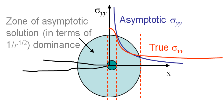
As seen in the earlier chapters, the Small Scale Yielding (SSY) assumption requires the process zone (region of inelastic deformations involving plastic flow, micro-fractures, void growth) to be confined to a very small region close to the crack tip, when compared to the size of the specimen. In that case, there exists a region in which the asymptotic solution is a good approximation of the real stress field, see Picture VII.1. Linear Elastic Fracture Mechanics (LEFM) theory could very well predict the fracture process in structures with a good accuracy.
As this will be discussed in this chapter and in the following one, the validity of this approach demands the conditions of a thick specimen (of thickness $t$), of a crack size ($a$) long enough, and of long enough other characteristic lengths such as the ligament ($L$), in order to neglect the size of the process zone:
\begin{equation} a, t, L > 2.5 \bigg(\frac{K_i}{\mathbf{\sigma}_p^0}\bigg) \label{eq:LEFMvalidity},\end{equation}
where $K_i$ is the relevant stress intensity factor (the toughness in the case of a crack propagation assessment, the current stress intensity factor in the case of a fatigue analysis), and $\mathbf{\sigma}_p^0$ is the material initial yield stress. If the expression (\ref{eq:LEFMvalidity}) is not satisfied, then the Linear Elastic Fracture Mechanics approach does not hold anymore and the effect of plasticity inside the process zone needs to be considered.
Cohesive Zone > Elastoplastic Behavior
Small deformations theory
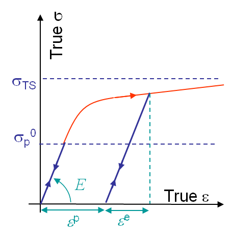
Considering a loading in 1D, once the stress $\sigma$ reaches the initial yield value $\mathbf{\sigma}_p^0$ the behavior is irreversible, and upon elastic unloading a permanent deformation ${\varepsilon}^\text{p}$ remains, as shown in Picture VII.2. During this irreversible plastic flow, the strain ${\varepsilon}$ has thus two contributions, the reversible or elastic one ${\varepsilon}^\text{e}$ and the irreversible or plastic one ${\varepsilon}^\text{p}$.
The generalization to the 3D case is based on the definition of a yield surface $ f\left(\mathbf{\sigma}\right) ≤0 $ , where $f<0$ defines the elastic region and $f=0$ defines the elasto-plastic one. Assuming the strains to be additive, i.e. that the strains remain small, one has
\begin{equation} d{\mathbf{\varepsilon}}=d{\mathbf{\varepsilon}^\text{e}}+d{\mathbf{\varepsilon}^\text{p}}\label{eq:addstrains}, \end{equation}
with
\begin{equation} d{\mathbf{\sigma}}=\mathcal{H}:d{\mathbf{\varepsilon}^\text{e}} \label{eq:dstress}.\end{equation}
The infinitesimal plastic strain increment should be normal to the yield surface to minimize the energy, yielding
\begin{equation} d{\mathbf{\varepsilon}^\text{p}}=d{\lambda} \frac{\partial{f}}{\partial{\mathbf{\sigma}}}\label{eq:dstrainp}, \end{equation}
where $\lambda$ is the amplitude of the plastic multiplier. Note that these equations have to be written under the form of infinitesimal increments as the material response is history dependent.
For J2-Plasticity, a von Mises yield surface can be considered, and reads in the case of isotropic hardening:
\begin{equation} f=\sqrt{\frac{3}{2} \mathbf{s}: \mathbf{s}}-\mathbf{\sigma}_p\left(\bar{\varepsilon}^\text{p}\right)\leq 0, \label{eq:fvonMises}\end{equation}which is written in terms of the deviatoric part of the stress tensor
\begin{equation} \mathbf{s}=\mathbf{\sigma} - \frac{\text{tr}(\mathbf{\sigma})}{3} \mathbf{I} ,\label{eq:sdev}\end{equation}
and in terms of the evolution of the yield stress $\mathbf{\sigma}_p\left(\bar{\varepsilon}^\text{p}\right)$ with the equivalent plastic deformation increment $d\bar{\varepsilon}^\text{p}=\sqrt{\frac{2}{3} d\mathbf{\varepsilon}^\text{p} : d\varepsilon^\text{p}} $.
From the definition Eq. (\ref{eq:sdev}) of the deviatoric stress tensor, one has the following relation
\begin{equation} \frac{\partial{\mathbf{s}_{ij}}}{\partial{\mathbf{\sigma}_{kl}}} =\frac{\partial({\mathbf{\sigma}_{ij}}-\frac{1}{3}\text{tr}(\mathbf{\sigma}){\delta_{ij}})}{\partial{\mathbf{\sigma}_{kl}}} =\frac{1}{2}{\delta_{ik}}{\delta_{jl}} + \frac{1}{2}{\delta_{il}}{\delta_{jk}} - \frac{1}{3}{\delta_{ij}}{\delta_{kl}}\label{eq:derivs}, \end{equation}
and the normal to the yield surface (\ref{eq:fvonMises}) of an isotropic elastic material becomes
\begin{equation} \frac{\partial f}{\partial \mathbf{\sigma}}=\sqrt{\frac{3}{2}} \frac{\mathbf{s}} {\sqrt{\mathbf{s}: \mathbf{s}}} \label{eq:normalvonMises}.\end{equation}
The normal flow rule (\ref{eq:dstrainp}) thus implies
\begin{equation} d \bar{\varepsilon}^\text{p} = \sqrt{\frac{2}{3} d\mathbf{\varepsilon}^\text{p} : d\varepsilon^\text{p}}=d{\lambda} \label{eq:dlambda}, \end{equation}
and thus for J2-plasticity
\begin{equation} d{\mathbf{\varepsilon}^\text{p}}=d \bar{\varepsilon}^\text{p} \sqrt{\frac{3}{2}} \frac{\mathbf{s}} {\sqrt{\mathbf{s}: \mathbf{s}}}\label{eq:dstrainpJ2}. \end{equation}
Existence of a potential for monotonic loading
As elasto-plastic material behaviors are history-dependent, an internal potential cannot be defined in the general case. However, in the case of monotonic and proportional loading, i.e. if all the stress components increase monotonically and proportionally to each other, the material can be seen as a non-linear elastic material and the existence of an internal potential is recovered.
Elastic-perfectly plastic material law
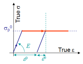
A perfectly plastic J2-material, characterized by the hardening parameter $h^\text{p} =\frac{\partial {\mathbf{\sigma}_p}}{\partial\bar{\varepsilon}^\text{p}}=0$, is first considered, see Picture VII.3.
Assuming the loading is monotonic and proportional, an internal potential $U$ can be defined during the plastic flow as,
\begin{equation} U=\frac{\mathbf{\varepsilon}^\text{e}:\mathcal{H}:\mathbf{\varepsilon}^\text{e}}{2}+\mathbf{\sigma}_p^0 \bar{\varepsilon}^\text{p}\label{eq:internalPotentialPP}. \end{equation}
Indeed, as $\mathbf{\varepsilon}^\text{e}=\mathbf{\varepsilon}-\mathbf{\varepsilon}^\text{p}$ differentiating this internal potential leads to
\begin{equation}
\partial_{\mathbf{\varepsilon}} U=\mathcal{H}:{\mathbf{\varepsilon}^\text{e}}
-\left(\mathcal{H}:\mathbf{\varepsilon}^\text{e}\right):\partial_{\mathbf{\varepsilon}} \mathbf{\varepsilon}^{\text{p}}+\mathbf{\sigma}_p^0
\partial_{\mathbf{\varepsilon}^{\text{p}}}\bar{\varepsilon}^\text{p}:\partial_{\mathbf{\varepsilon}}{\varepsilon}^{\text{p}}.\label{eq:derivPP1}
\end{equation}
Under the assumption of monotonic and proportional loading, the equivalent plastic strain reads $\bar{\varepsilon}^\text{p} = \sqrt{\frac{2}{3} \mathbf{\varepsilon}^\text{p}:\mathbf{\varepsilon}^\text{p}}$, and allows Eq. (\ref{eq:dstrainpJ2}) to be rewritten as
\begin{equation} \mathbf{\varepsilon}^\text{p} = \bar{\varepsilon}^\text{p} \frac{\partial f}{\partial \mathbf{\sigma}}= \sqrt{\frac{3}{2}} \bar{\varepsilon}^\text{p} \frac{\mathbf{s}} {\sqrt{\mathbf{s}:\mathbf{s}}} \label{eq:derivPP2}, \end{equation}
which yields
\begin{equation} \mathbf{\varepsilon}^\text{p} = \bar{\varepsilon}^\text{p} \frac{\partial f}{\partial \mathbf{\sigma}}= \sqrt{\frac{3}{2}} \bar{\varepsilon}^\text{p} \frac{\mathbf{s}} {\sqrt{\mathbf{s}:\mathbf{s}}}. \label{eq:derivPP3} \end{equation}
Therefore, as $\bar{\varepsilon}^\text{p} = \sqrt{\frac{2}{3} \mathbf{\varepsilon}^\text{p}:\mathbf{\varepsilon}^\text{p}}$, one has
\begin{equation} \partial_{{\mathbf{\varepsilon}}^\text{p}}\bar{\varepsilon}^\text{p}=\sqrt{\frac{2}{3}}\frac{{\mathbf{\varepsilon}}^\text{p}}{\sqrt{{\mathbf{\varepsilon}}^\text{p}:{\mathbf{\varepsilon}}^\text{p}}}=\sqrt{\frac{2}{3}}\frac{\bar{\varepsilon}^\text{p}\sqrt{\frac{3}{2}}\frac{\mathbf{s}}{\sqrt{\mathbf{s}:\mathbf{s}}}}{\bar{\varepsilon}^\text{p}\sqrt{\frac{3}{2}}\sqrt{\frac{\mathbf{s}:\mathbf{s}}{\mathbf{s}:\mathbf{s}}}}=\sqrt{\frac{2}{3}} \frac{\mathbf{s}}{\sqrt{\mathbf{s}:\mathbf{s}}}. \label{eq:derivPP4}\end{equation}
Moreover, as ${\mathbf{\varepsilon}}^\text{p}$ is deviatoric, the two first terms of Eq. (\ref{eq:derivPP1}) become
\begin{equation} \mathcal{H}:{\mathbf{\varepsilon}^\text{e}}-\left(\mathcal{H}:{\mathbf{\varepsilon}^\text{e}}\right):\partial_{\mathbf{\varepsilon}}{\mathbf{\varepsilon}}^{\text{p}}=\mathbf{\sigma}-\mathbf{s}:\partial_{\mathbf{\varepsilon}}\mathbf{\varepsilon}^{\text{p}}.\label{eq:derivPP5} \end{equation}The von Mises surface definition (\ref{eq:fvonMises}) for a perfectly plastic material ($\mathbf{\sigma}_p^0=\mathbf{\sigma}_p$) leads to
\begin{equation} \mathbf{\sigma}_p^0 \sqrt{\frac{2}{3}} \frac{\mathbf{s}}{\sqrt{\mathbf{s}:\mathbf{s}}}=\mathbf{s}. \label{eq:derivPP6}\end{equation}
Eventually, combining Eqs. (\ref{eq:derivPP4}-\ref{eq:derivPP6}) allows rewriting Eq. (\ref{eq:derivPP1}) as
\begin{equation} \partial_{\mathbf{\varepsilon}}U=\mathbf{\sigma}-\mathbf{s}:\partial_\mathbf{\varepsilon}\mathbf{\varepsilon}^\text{p}+\mathbf{s}:\partial_\mathbf{\varepsilon}\mathbf{\varepsilon}^\text{p}=\mathbf{\sigma}.\label{eq:derivPP7} \end{equation}
This demonstrates the existence of an internal potential for perfectly plastic material, as if there is no unloading, the stress still derives from a potential.
Material law for J2-plasticity with non-linear hardening
In order to consider more general elasto-plastic behaviors, a power hardening law is now considered
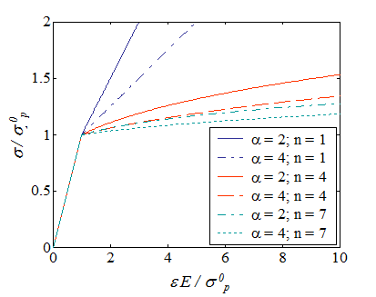
\begin{equation} \mathbf{\sigma}_p \left(\bar{\varepsilon}^\text{p}\right) = \mathbf{\sigma}_p^0{\bigg(\frac{\bar{\varepsilon}^\text{p}}{\frac{{\alpha}{\sigma}_p^0}{E}}+1\bigg)}^\frac{1}{n}.\label{eq:powerlaw} \end{equation}
This hardening law is characterized by the parameters $\alpha$ and $n$ whose variations lead to different material responses as shown in Picture VII.4. In particular, when $n\rightarrow\infty$, a perfectly plastic behavior is recovered. The term $\frac{{\sigma}_p^0}{E}$ in Eq. (\ref{eq:powerlaw}) represents the elastic deformation of the specimen at initial yield.
The relation (\ref{eq:powerlaw}) can be inverted in order to express the evolution of the equivalent plastic strain $\bar{\varepsilon}^\text{p}$ in terms of the current yield stress ${\sigma}_p$, with
\begin{equation} \bar{\varepsilon}^\text{p} ={\frac{{\alpha}{\mathbf{\sigma}_p^0}}{E}}{\bigg(\frac{{\sigma}_p}{{\sigma}_p^0}\bigg)}^n-\frac{{\alpha}{{\sigma}_p^0}}{E}.\label{eq:powerlawinverted} \end{equation}
In order to investigate the evolution of the plastic strain tensor $\mathbf{\varepsilon}^\text{p}$ during the plastic flow, the power law (\ref{eq:powerlawinverted}) is first differentiated, leading to
\begin{equation} d\bar{\varepsilon}^{\text{p}}=\frac{n{\alpha}{\sigma}_p^0}{E} {\bigg(\frac{{\sigma}_p}{{\sigma}_p^0}\bigg)}^{n-1} \frac{d{\sigma}_p}{{\sigma}_p^0}\label{eq:derivationpowerlaw1}, \end{equation}
which allows Eq. (\ref{eq:dstrainpJ2}) to be rewritten using Eq. (\ref{eq:fvonMises}) as
\begin{equation}
d\mathbf{\varepsilon}^\text{p}=\sqrt{\frac{3}{2}}\frac{\mathbf{s}}{\sqrt{\mathbf{s}:\mathbf{s}}}\frac{n{\alpha}{\sigma}_p^0}{E}{\bigg(\frac{{\sigma}_p}{{\sigma}_p^0}\bigg)}^{n-1}\frac{d{\sigma}_p}{{\sigma}_p^0}=
\frac{3}{2}\frac{\mathbf{s}}{{\sigma}_p^0}\frac{n{\alpha}{\sigma}_p^0}{E}{\bigg(\frac{{\sigma}_p}{{\sigma}_p^0}\bigg)}^{n-2}\frac{d{\sigma}_p}{{\sigma}_p^0}
.
\label{eq:derivationpowerlaw2}\end{equation}
Assuming a monotonic and proportional loading, the incremental form can be substituted by the finite one and the plastic strain tensor is directly obtained by combining Eqs. (\ref{eq:dstrainpJ2}) and (\ref{eq:powerlawinverted}) as,
\begin{equation}
\mathbf{\varepsilon}^\text{p}=\bar{\varepsilon}^\text{p}\sqrt{\frac{3}{2}}\frac{\mathbf{s}}{\sqrt{\mathbf{s}:\mathbf{s}}}=
\bigg[\frac{{\alpha}{\sigma}_p^0}{E}{\bigg(\frac{{\sigma}_p}{{\sigma}_p^0}\bigg)}^n-\frac{{\alpha}{\sigma}_p^0}{E}\bigg]
\sqrt{\frac{3}{2}}\frac{\mathbf{s}}{\sqrt{\mathbf{s}:\mathbf{s}}},\label{eq:derivationpowerlaw3}
\end{equation}
or again, by using Eq. (\ref{eq:fvonMises}), as
\begin{equation} \mathbf{\varepsilon}^\text{p}=\bigg[\frac{{\alpha}{\sigma}_p^0}{E}{\bigg(\frac{{\sigma}_p}{{\sigma}_p^0}\bigg)}^{n-1}-\frac{{\alpha}\left({\sigma}_p^0\right)^2}{E{\sigma}_p}\bigg]\frac{3}{2}\frac{\mathbf{s}}{{\sigma}_p^0} . \label{eq:derivationpowerlaw4}\end{equation}
\begin{equation} U=\int_0^{\mathbf{\varepsilon}}\mathbf{\sigma}:d\mathbf{\varepsilon'}=\int_0^{\mathbf{\varepsilon}^\text{e}}\mathbf{\sigma}:d\mathbf{\varepsilon}^\text{e'}+\int_0^{\mathbf{\varepsilon}^\text{p}}\mathbf{\sigma}:d\mathbf{\varepsilon}^\text{p'} =\int_0^{\mathbf{\varepsilon}^\text{e}}\mathbf{\varepsilon}^\text{e'}:\mathcal{H}:d\mathbf{\varepsilon}^\text{e'}+\int_0^{\mathbf{\varepsilon}^\text{p}}\mathbf{s}:d\mathbf{\varepsilon}^\text{p'},\label{eq:derivationpowerlaw5} \end{equation}
as the plastic deformation tensor is deviatoric. Using Eq. (\ref{eq:derivationpowerlaw2}) and Eq. (\ref{eq:fvonMises}), this last relation reads
\begin{equation} U=\frac{\mathbf{\varepsilon}^\text{e}:\mathcal{H}:\mathbf{\varepsilon}^\text{e}}{2}+\int_{{\sigma}_p^0}^{{\sigma}_p}\mathbf{s}:\frac{3}{2}\frac{\mathbf{s}}{{\sigma}_p^0}\frac{n{\alpha}{\sigma}_p^0}{E}\bigg(\frac{{\sigma}_p'}{{\sigma}_p^0}\bigg)^{n-2}\frac{d{\sigma}_p'}{{\sigma}_p^0} =\frac{\mathbf{\varepsilon}^\text{e}:\mathcal{H}:\mathbf{\varepsilon}^\text{e}}{2}+\int_{{\sigma}_p^0}^{{\sigma}_p}\frac{n{\alpha}{\sigma}_p^0}{E}{\bigg(\frac{{\sigma}'_p}{{\sigma}_p^0}\bigg)}^n d{\sigma}'_p.\label{eq:derivationpowerlaw6} \end{equation}
Eventually, performing the integral and using Eq. (\ref{eq:powerlaw}) yield the final expression of the internal potential
\begin{equation} U=\frac{\mathbf{\varepsilon}^\text{e}:\mathcal{H}:\mathbf{\varepsilon}^\text{e}}{2}+\frac{n{\alpha}\left({\sigma}_p^0\right)^2}{E\left(n+1\right)}\bigg[{\bigg(\frac{\bar{\varepsilon}^\text{p}}{{\frac{{\alpha}{\sigma}_p^0}{E}}}+1\bigg)}^\frac{n+1}{n}-1\bigg]. \label{eq:derivationpowerlaw7}\end{equation}
![]()