
Numerical Methods > Ductile materials
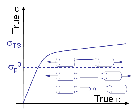
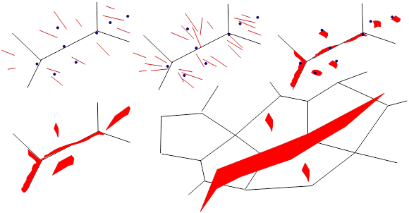
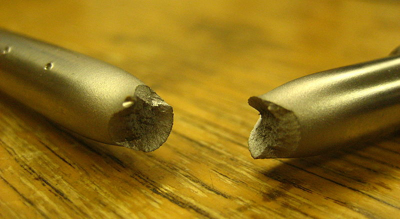
The previously described methods were developed under the LEFM and SSY assumptions. The failure mechanism of ductile material is different from the brittle and SSY materials: important plastic deformations take place prior to the (macroscopic) failure of the specimen, see Picture VI.19. The plastic deformations result from dislocations motion which pile up at inclusions, grain boundaries ... leading to the nucleation and growth of micro-voids, see Picture VI.20. Fially, micro-voids grow and coalesce to form micro-cracks. This failure mechanisms results in typical failure surfaces as shown in Picture VI.21.
The numerical model ought to represent this failure mode: micro-voids nucleation, growth, and coalescence. Toward this end, continuum damage mechanics (CDM) models the progressive degradation of the material and the effects of the porosity on its behavior.
Introduction to Chaboche's continuum damage mechanics model
As there are voids in the material, when considering a material section, only a reduced surface is balancing the traction, modifying the apparent constitutive behavior.
Damage definition
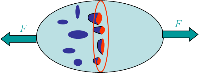
Let us consider a body with under tension $F$, see Picture VI.22. For a virgin material section $S$ free of voids the stress is equivalent to
\begin{equation} \sigma_{xx}^{virgin} = \frac{F}{S} = \sigma_{xx}. \end{equation}
However, in the presence of cavities, two stress measures can be defined. The first one is the apparent stress, which is computed ignoring the micro-voids:
\begin{equation} \sigma_{xx} = \frac{F}{S}. \end{equation}
The second one, the effective stress, corresponds to the stress actually sustained by the material remaining once the voids have been removed. This effective stress can be related to the apparent one through the porosity. The damage is here defined as the porosity: the ratio between the voids section $S^{holes}$ and the total apparent surface $S$, i.e. $D = \frac{S^{holes}}{S}$, see Picture VI.22. The effective (or damaged) surface is actually the section of material that can sustain the loading $F$: $\hat{S} = S - S^{holes} = (1-D)S$. The effective stress inside the material thus reads
\begin{equation} \hat{\sigma}_{xx} = \frac{F}{S(1-D)} = \frac{\sigma_{xx}}{1-D}. \end{equation}
The resulting deformation can be obtained from the Hooke's law expressed in terms of the stress which effectively balances the loading: the effective stress:
\begin{equation} \varepsilon_{xx} = \frac{\hat{\sigma}_{xx}}{E} = \frac{\sigma_{xx}}{E(1-D)}. \end{equation}
As a result, the material elastic behavior in terms of the apparent stress tensor is obtained as if the Hooke's law was multiplied by $(1-D)$.
This approach can be extended to isotropic 3D linear elasticity in a similar way:
\begin{equation} \mathbf{\sigma} = (1-D) \mathbf{\mathcal{H}} : \mathbf{\varepsilon}. \label{eq:sigDevo}\end{equation}
A failure criterion can then be chosen based on the damage: $D = D_C$ with $0 < D_c < 1$ a critical damage value.
To complete the framework, the evolution of the porosity with the deformations should be defined.
Evolution of damage $D$ for isotropic elasticity
Damage has been introduced, but a constitutive relation is required in order to describe its evolution. This can be done by defining a damage surface:
\begin{equation} f(\mathbf{\varepsilon}, D) = (1-D) \frac{\mathbf{\varepsilon} : \mathbf{\mathcal{H}}: \mathbf{\varepsilon}}{2} - Y_C \leq 0, \label{eq:Devo} \end{equation}
where $Y_C$ is an energy related deformation threshold. The damage evolution is then defined by the condition
\begin{equation}f\dot{D} = 0,\end{equation}
which is interpreted by
- Either $f=0$ and the damage increases: $\dot{D} > 0$, or
- $f < 0$ and the damage remains constant: $\dot{D} = 0$.
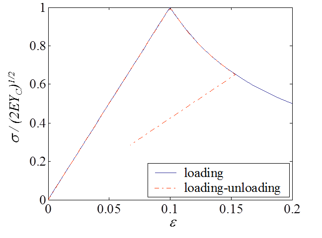
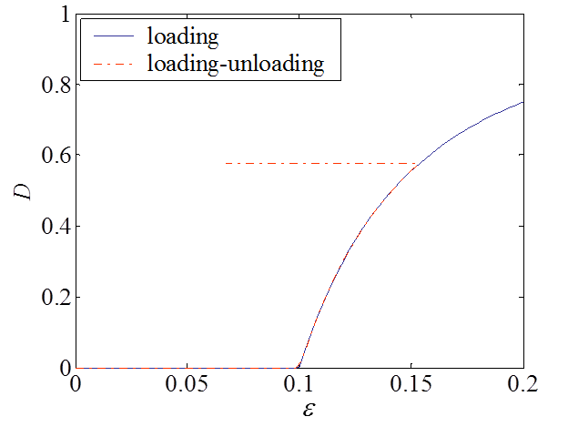
An example of material response for a damage-enhanced elastic material obeying to Eqs. (\ref{eq:sigDevo}- \ref{eq:Devo}) is illustrated in Picture VI.23 and Picture VI.24. In this application, $Y_C$ is taken such that damage appears for $\varepsilon = 0.1$. One can see than once this stress is reached, the material exhibits a softening with the damage evolution during the loading response. Unloading occurs at constant damage and corresponds to a reduced elastic slope.
Gurson's model
However, this model does not represent the evolution of the damage related to the plastic flow. Plasticity combined to porosity evolution plays a key role in the damaging process for ductile materials and has to be considered in the model. Toward this end, Gurson has developed a dedicated damage-enhanced elasto-plasticity model.
The multi-scale model
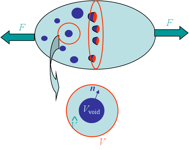
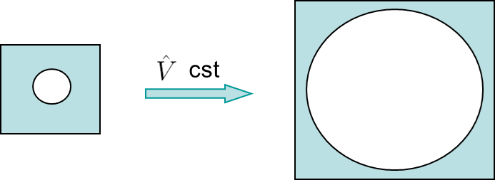
The Gurson's model was derived in 1977. It assumes that the material obeys to a rigid-perfectly-plastic assumption and embeds initial spherical micro-voids. A spherical volume $V$ representative of the porous material is extracted and is illustrated in Picture VI.25. This volume $V$ embeds a spherical micro-void $V_{\text{void}}$ such that the effective material part of the volume $V$ is $\hat{V}=V-V_{\text{void}}$. The porosity $f_V$ is thus defined as the fraction of voids in the total volume of the representative volume:
\begin{equation} f_V = \dfrac{V_{\text{void}}}{V} = 1 - \dfrac{\hat{V}}{V}.\label{eq:GursonPorosity}\end{equation}
The formulation is multi-scale. We can thus define the fields at two different scales:
- The macroscopic strain and stress tensors, respectively $\mathbf{\varepsilon}$ and $\mathbf{\sigma}$, are the apparent tensors at the structural level obtained by considering the homogenized values on the representative volume $V$;
- The microscopic strain and stress tensors, respectively $\hat{\mathbf{\varepsilon}}$ and $\hat{\mathbf{\sigma}}$, are the tensors distribution within the representative volume $V$, and which are thus not constant in the representative volume $V$.
The relations between the different microscopic and macroscopic tensors are obtained by following a homogenization process.
On the one hand, the relation between the macroscopic and microscopic strain (rate) tensors follows a volume averaging (the homogenization step) on the representative volume $V$:
\begin{equation} \dot{\mathbf{\varepsilon}} = \dfrac{1}{V} \int_V \mathbf{\dot{\hat{\varepsilon}}} dV = \dfrac{1}{V} \int_{\hat{V}} \dot{\hat{\mathbf{\varepsilon}}} dV + \dfrac{1}{V} \int_{V_{\text{void}}} \dot{\hat{\mathbf{\varepsilon}}} dV, \label{eq:Gurson1}\end{equation}
where we have used the decomposition of the representative volume $V$ into the effective part $\hat{V}$ and the porosity part $V_{\text{void}}$. Note that, although the stress vanishes in the voids, this is not the case of the strain as the voids deform with the loading. Using the Gauss theorem, as $\hat{\mathbf{\varepsilon}}=\frac{1}{2}\left(\mathbf{\nabla}\otimes\hat{\mathbf{u}}+\hat{\mathbf{u}}\otimes\mathbf{\nabla}\right)$, this last relation (\ref{eq:Gurson1}) becomes
\begin{equation} \dot{\mathbf{\varepsilon}} = \dfrac{1}{V} \int_V \dot{\hat{\mathbf{\varepsilon}}} dV = \dfrac{1}{V} \int_{\hat{V}} \dot{\hat{\mathbf{\varepsilon}}} dV + \dfrac{1}{2V} \int_{S_{\text{void}}} \left[\dot{\hat{\mathbf{u}}} \otimes \mathbf{n} + \mathbf{n} \otimes \dot{\hat{\mathbf{u}}}\right] dV,\label{eq:Gurson2} \end{equation}
where $ \mathbf{n}$ is the outward unit normal to the void.
On the other hand, the microscopic stress tensor $\hat{\mathbf{\sigma}}$ is related to the microscopic strain rate tensor $\dot{\hat{\mathbf{\varepsilon}}}$ through an energy rate
\begin{equation} \hat{\mathbf{\sigma}} = \dfrac{\partial \dot{\hat{W}}}{\partial \dot{\hat{\mathbf{\varepsilon}}}}.\label{eq:Gurson3}\end{equation}
The energy rate has to be conserved between the microscopic and macroscopic levels,
\begin{equation} \dot{W} \left( \dot{\mathbf{\varepsilon}} \right) = \dfrac{1}{V} \int_{V} \dot{\hat{W}} \left( \dot{\hat{\mathbf{\varepsilon}}} \right) dV= \dfrac{1}{V} \int_{\hat{V}} \dot{\hat{W}} \left( \dot{\hat{\mathbf{\varepsilon}}} \right) dV,\label{eq:Gurson4} \end{equation}
as the microscopic energy rate $\dot{\hat{W}}$ vanishes in the voids. Combining (\ref{eq:Gurson3}) and (\ref{eq:Gurson4}) leads to the expression of the macroscopic stress
\begin{equation} \mathbf{\sigma} = \frac{\partial \dot{W}}{\partial \dot{\mathbf{\varepsilon}}} = \dfrac{1}{V} \int_{\hat{V}} \dfrac{\partial \dot{\hat{W}}}{\partial \dot{\hat{\mathbf{\varepsilon}}}}: \dfrac{\partial \dot{\hat{\mathbf{\varepsilon}}}}{\partial \dot{\mathbf{\varepsilon}}} dV = \dfrac{1}{V} \int_{\hat{V}} \hat{\mathbf{\sigma}} : \dfrac{\partial \dot{\hat{\mathbf{\varepsilon}}}}{\partial \dot{\mathbf{\varepsilon}}} dV.\label{eq:Gurson5} \end{equation}
The multiscale model corresponds to defining the macroscopic $\mathbf{\sigma}-\mathbf{\varepsilon}$ relation through the resolution of the equations (\ref{eq:Gurson2}) and (\ref{eq:Gurson5}) for a given microscopic constitutive behavior (\ref{eq:Gurson3}).
Gurson's apparent yield surface
Gurson has solved this multiscale model assuming a rigid-perfectly-plastic microscopic behavior (\ref{eq:Gurson3}) at the microscopic scale. Since the material in the effective part $\hat{V}$ follows a rigid-perfectly plastic material law, the elastic deformations are neglected in this original model.
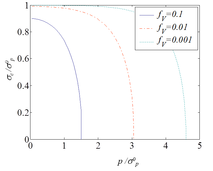
The result of this multiscale model is the definition of an apparent macroscopic yield surface which depends on the microscopic porosity $f_V$:
\begin{equation} f(\mathbf{\sigma}) = \left( \dfrac{\sigma_e}{\sigma^0_p} \right)^2 + 2 f_V \cosh{\left( \dfrac{\text{tr}(\mathbf{\sigma})}{2 \sigma_p^0}\right)} - f_V^2 -1 \leq 0,\label{eq:GursonYieldSurface} \end{equation}
with the equivalent macroscopic von Mises stress $\mathbf{\sigma}_e = \sqrt{\dfrac{3}{2} \mathbf{s}:\mathbf{s}}$, and the effective material yield stress $\sigma^0_p$.
This yield function is illustrated in Picture VI.26 and has the following properties:
- If $f_V = 0$, the usual J2-plasticity yield function is recovered;
- If $f_V \neq 0$, the yield surface is pressure-dependent;
- If $f_V \neq 0$, a hydrostatic stress state ($\sigma_e = 0$, $\text{tr}\left(\mathbf{\sigma}\right)=3p$) can induce plasticity, and the yielding pressure is evaluated as follows
- Indeed (\ref{eq:GursonYieldSurface}) is rewritten: $f_V^2 -2 f_V \cosh{\frac{3p}{2\sigma^0_p}} + 1 \leq 0$;
- Plastic flow thus occurs for $f_V = \cosh{\frac{3p}{2\sigma^0_p}} \pm \sinh{\frac{3p}{2\sigma^0_p}}$ ;
- Or $f_V = \dfrac{\exp{\left( \frac{3p}{2\sigma^0_p}\right)} + \exp{\left(-\frac{3p}{2\sigma^0_p} \right)} \pm \exp{\left( \frac{3p}{2\sigma^0_p} \right)} \mp \exp{\left(- \frac{3p}{2\sigma^0_p} \right)} }{2} = \exp{\pm \frac{3p}{2 \sigma_p^0}}$;
- This last results can be reformulated as $\dfrac{3p}{2 \sigma_p^0} = \pm \ln{f_V}$ ;
- When $f_V = 0$, the sign $-$ has to be chosen as a pressure cannot induce plasticity, so that the yielding pressure is $p = - \dfrac{2 \sigma_p^0\ln{f_V}}{3}$.
The yield surface (\ref{eq:GursonYieldSurface}) is associated with a normal flow rule, and the problem is thus completed at the macroscale by
\begin{equation} \begin{cases} f \dot{\lambda} &=& 0,\\ \dot{\mathbf{\varepsilon}}^p &=& \dot{\lambda} \dfrac{\partial f}{\partial \mathbf{\sigma}}>0.\end{cases}\label{eq:GursonFlow} \end{equation}
The Gurson's porosity plasticity model is thus defined at a given porosity $f_V$ by the equations (\ref{eq:GursonYieldSurface}) and (\ref{eq:GursonFlow}). In the next section, the evolution of the porosity during the plastic flow is studied.
Porosity evolution
To complete the set of equations (\ref{eq:GursonYieldSurface}) and (\ref{eq:GursonFlow}), the evolution of the porosity during the plastic flow is computed by evaluating the relation between the effective and apparent volumes, see Picture VI.27. The effective volume $\hat{V}$ is constant as elastic deformations were neglected in the effective material (rigid-perfectly-plastic microscopic behavior) and as plastic deformations are isochoric (at the microscopic scale). The effective volume is related to the apparent volume $V$ through the definition of the porosity (\ref{eq:GursonPorosity}): $\hat{V}=(1-f_V) V$. As the effective volume is constant, the porosity and the macroscopic volume variation are related by:
\begin{equation} 0 = (1-f_V) dV - df_V V. \end{equation}
Since the apparent volume variation $dV$ corresponds to the trace of the macroscopic deformation tensor, and since the elastic strains are neglected, this last relation is rewritten
\begin{equation} \dot{f_V} = (1-f_V)\dfrac{\dot{V}}{V} = (1-f_V) \text{tr}(\dot{\mathbf{\varepsilon}}) = (1-f_V) \text{tr}(\dot{\mathbf{\varepsilon}}^p) .\label{eq:GursonPorosityEvolution}\end{equation}
This completes the original Gurson's formulation for a rigid perfectly-plastic microscopic material behavior. This original model also assumes an initial porosity as no new voids nucleation is modeled. Voids interaction and coalescence are also ignored.
Gurson's model improvements
To address some of the limitations resulting from the assumptions of the original Gurson's formulation, several improvements were proposed in the literatures. Some of them are described here below, without being exhaustive.
Microscopic material behavior with isotropic hardening
During the microscopic plastic flow, the effective von Mises $\hat{\sigma}_e$ is no longer equal to a constant $\sigma_p^0$, but to the yield stress $\sigma_p(\hat{\bar{\varepsilon}}^p)$, which depends on the equivalent microscopic plastic strain $\hat{\bar{\varepsilon}}^p$ through an isotropic hardening model. As a result, the yield criterion (\ref{eq:GursonYieldSurface}) becomes
\begin{equation} f(\mathbf{\sigma}) = \left( \dfrac{\sigma_e}{\sigma_p(\hat{\bar{\varepsilon}}^p)} \right)^2 + 2 f_V \cosh{\left( \dfrac{tr(\mathbf{\sigma})}{2 \sigma_p(\hat{\bar{\varepsilon}}^p)}\right)} - f_V^2 -1 \leq 0. \label{eq:GursonHardeningYieldSurface} \end{equation}
The equivalent plastic strain $\sigma_p(\hat{\bar{\varepsilon}}^p)$ does evolve in terms of the matrix plastic strain $\hat{\bar{\varepsilon}}^p$ and not in terms of the macroscopic plastic strain $\bar{\varepsilon}^p$. To define the matrix plastic strain the conservation of the dissipated energies is enforced, leading to
\begin{equation} (1-f_V) \sigma_p \left( \hat{\bar{\varepsilon}}^p\right) \dot{\hat{\bar{\varepsilon}}^p} = \mathbf{\sigma} : \dot{\mathbf{\varepsilon}^p}. \end{equation}
Voids nucleation
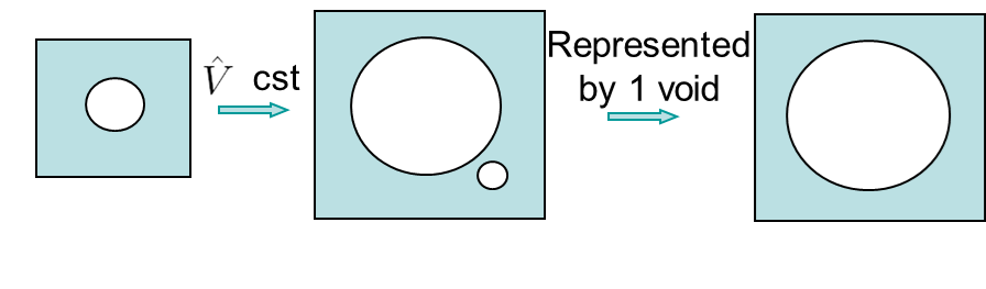
The porosity evolution has two origins, see Picture VI.28:
-
The evolution related to the apparent deformation of the volume element combined to the incompressible nature of the microscopic plastic flow in the matrix material, as stated by equation (\ref{eq:GursonPorosityEvolution});
-
The creation of new voids $\dot{f}_{\text{nucl}}$, also called nucleation, resulting from the material loading.
The combination of the two effects allows replacing (\ref{eq:GursonPorosityEvolution}) by
\begin{equation} \dot{f_V} = (1-f_V) \text{tr}(\dot{\mathbf{\varepsilon}}^p) + \dot{f}_{\text{nucl}}. \end{equation}
The nucleation rate can be obtained by different models. One of them relates the nucleation rate to the microscale plastic strain, $\dot{f}_{\text{nucl}} = A(\hat{\bar{\varepsilon}}^p) \dot{\hat{\bar{\varepsilon}}^p}$.
Note that the porosity $f_V$ is a representation of the different microscopic voids. In the original Gurson's model the microscopic voids are treated as a single one within a representative volume, see Picture VI.28.
Voids interaction
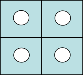
As previously stated, the original Gurson's model considers the microscopic voids as a single hole within a representative volume, see Picture VI.28. In 1981, Tvergaard added the voids interaction effect to the Gurson's model. While voids are considered as isolated in the original version, they are now interacting with each other, see Picture VI.29. The yield function (\ref{eq:GursonHardeningYieldSurface}) is modified into
\begin{equation} f(\mathbf{\sigma}) = \left( \dfrac{\sigma_e}{\sigma_p(\hat{\bar{\varepsilon}}^p)} \right)^2 + 2q f_V \cosh{\left( \dfrac{tr(\mathbf{\sigma})}{2 \sigma_p(\hat{\bar{\varepsilon}}^p)}\right)} - q^2f_V^2 -1 \leq 0. \label{eq:interactionGursonHardeningYieldSurface} \end{equation}
The presence of neighboring voids decreases the maximal loading as the stress distribution changes, which is modeled by considering $1 < q < 2$, depending on the hardening exponent.
Voids coalescence
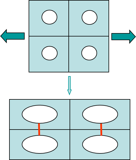
Tvergaard and Needleman further improved the voids interaction model in 1984. Physically, when two voids are close to each other the material loses capacity of sustaining the loading, see Picture VI.30. In order to assess whether voids can coalesce, a threshold porosity $f_C$ is defined, and voids start to merge when $f_V \sim f_C$. Then, if $f_V$ still increases, the material is unable to sustain any more loading. To model this effect, an effective porosity is used in the yield function, and (\ref{eq:interactionGursonHardeningYieldSurface}) is replaced by
\begin{equation} f(\mathbf{\sigma}) = \left( \dfrac{\sigma_e}{\sigma_p(\hat{\bar{\varepsilon}}^p)} \right)^2 + 2q f_V^* \cosh{\left( \dfrac{tr(\mathbf{\sigma})}{2 \sigma_p(\hat{\bar{\varepsilon}}^p)}\right)} - \left(q^2f_V^*\right)^2 -1 \leq 0, \label{eq:colescenceGursonHardeningYieldSurface} \end{equation}
where the effective porosity is defined by
\begin{equation} f_V^* = \begin{cases} f_V &\text{ if }& f_V < f_C, \\ f_C + \dfrac{f_F^*-f_C}{f_F-f_C}(f_V-f_C) &\text{ if }& f_V > f_C, \end{cases} \end{equation}
with $f_C$ the critical porosity at voids coalescences, $F_f$ the critical porosity at ductile failure, and $F_f$ its corrected effective value.Application of Damage models
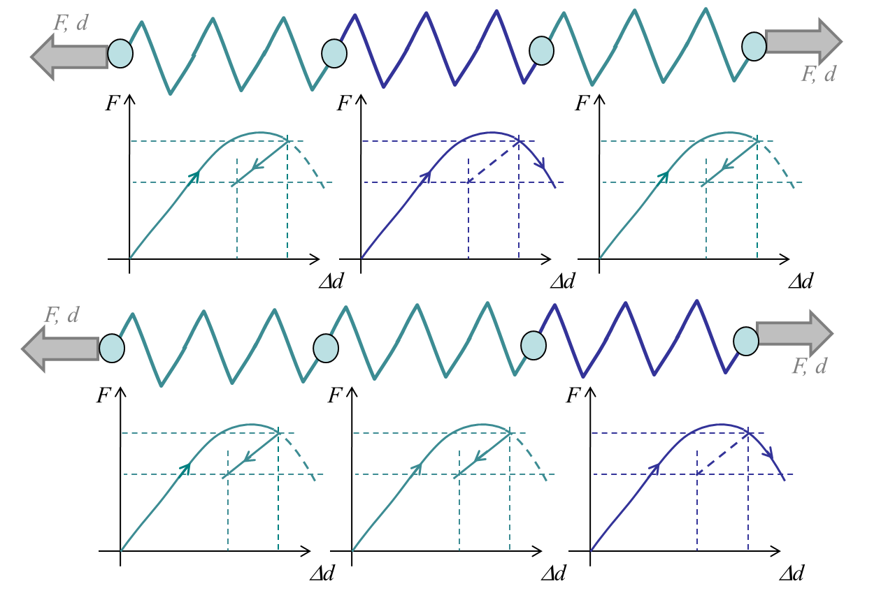
One of the main problems with continuum damage models is that during the strain softening part of the curves, i.e. when the stress decreases with the strain, the problem becomes ill-posed. The continuum mechanics equations lose their ellipticity, and the solution is no longer unique. For example, let us consider the system of three springs reported in Picture VI.31, and let us consider a displacement increment during the strain softening part. It can be seen that to reach a constant force or stress along the three springs, only one has to follow the irreversible loading part (the blue spring). The two other (green) springs can follow an elastic unloading. However, the irreversibly loaded (blue) spring can be any of the three ones. For a constant displacement $d$, one, two, or the three springs could also be along the irreversible loading part, yielding different forces $F$. In practice this has several effects:
- The problem is mesh dependent: when changing the mesh the solution changes (the blue spring can be any of the three elements);
- There is no unique solution: depending on the numerical error one element or an other one will be irreversibly loaded (one, two, or three elements can be irreversibly loaded);
- There is a localization issue: all the deformation could localize in a single element (here the blue spring).
Continuum damage model thus cannot be used during the softening response, unless they are formulated in a non-local way. With non-local approaches, a material length-scale is introduced in the model damage-related internal variables are averaged in volumes defined by this length-scale.
![]()