
Asymptotic Solution > Mode III (shearing) and summary
Mode III
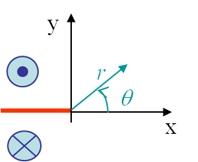
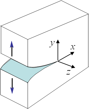
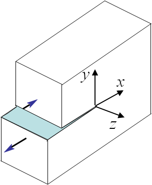
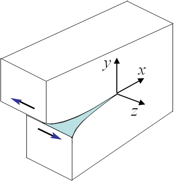
The boundary conditions associated to the third loading mode, see Picture II.26, were found to be
\begin{equation}\begin{cases} \mathbf{\sigma}_{xx} = \mathbf{\sigma}_{xy} = \mathbf{\sigma}_{yy} = \mathbf{\sigma}_{zz} = 0 \\ \mathbf{u}_x = \mathbf{u}_y = 0 \\ \mathbf{u}_z (\theta) = -\mathbf{u}_z (-\theta) \end{cases}.\label{eq:bcModeIII}\end{equation}
Resolution method
As the loading is out-of-plane, the resolution method differs from the two other modes. By definition of the strain tensor, one has
\begin{equation} \mathbf{\varepsilon}_{\alpha z}= \frac{1}{2}\mathbf{u}_{z,\alpha}\label{eq:epsModeIII}, \end{equation}
and the stress field directly derives from the Hooke's law
\begin{equation} \mathbf{\sigma}_{\alpha z} = \frac{E}{1+\nu}\mathbf{\varepsilon}_{\alpha z}=\frac{E}{2\left(1+\nu\right)}\mathbf{u}_{z,\alpha}.\label{eq:HookeModeIII}\end{equation}
The linear momentum equation $\nabla\cdot \mathbf{\sigma}=0$ simplifies in the case of pure shearing into $\mathbf{\sigma}_{\alpha z,\alpha} = 0$ and (\ref{eq:HookeModeIII}) yields
\begin{equation}
\nabla^2 \mathbf{u}_z = 0.\label{eq:LaplacianModeIII}
\end{equation}
As the Laplace's equation is satisfied, $\mathbf{u}_z$ is the imaginary part of a function $z(\zeta)$, see previous section, and
\begin{equation} \mathbf{u}_z = \mathcal{I}\left(z\left(\zeta\right)\right).\label{eq:cauchyRiemannModeIII} \end{equation}
This means that any choice of a complex function $z\left(\zeta\right)$ satisfies the linear elastic problem, as long as the BCs are also satisfied. Because of the discontinuity of the solution in $\theta=\pm \pi$, see Picture II.26, an obvious choice is
\begin{equation} z = \sum_{\lambda} C r^\lambda \exp{\left(i\theta\lambda\right)}\label{eq:zModeIII}, \end{equation}
with a real constant $C$ associated to each $\lambda$. Indeed
\begin{equation} \mathbf{u}_z = \mathcal{I}\left(z\left(\zeta\right)\right) = \sum_{\lambda} C r^\lambda \sin{\theta\lambda} ,\label{eq:uModeIIItmp} \end{equation}
is anti-symmetric, so it satisfies $\mathbf{u}_z (\theta) = -\mathbf{u}_z (-\theta)$, and has a discontinuity in $\theta=\pm\pi$ if the value of $\lambda=\frac{1}{2}$ is included in the series. For the displacement to remain finite, the series will be limited to $\lambda\geq 0$.
The strain field is obtained from (\ref{eq:epsModeIII}) -remembering that $\partial_x=\cos{\theta}\partial_r-\frac{\sin{\theta}}{r}\partial_\theta$ and $\partial_x=\sin{\theta}\partial_r+\frac{\cos{\theta}}{r}\partial_\theta$- and reads
\begin{equation}\begin{cases}
\mathbf{\varepsilon}_{x z} =\sum_{\lambda}\left[ \frac{C}{2}\lambda \cos{\theta}
r^{\lambda-1}\sin{\left(\theta\lambda\right)} - \frac{C}{2} \sin{\theta}
r^{\lambda-1}\lambda\cos{\left(\lambda\theta\right)}\right] =\sum_{\lambda} \frac{C}{2} \lambda
r^{\lambda-1} \sin{\left[\left(\lambda-1\right)\theta\right]}\\ \mathbf{\varepsilon}_{y z} = \sum_{\lambda} \left[\frac{C}{2}\lambda \sin{\theta}
r^{\lambda-1}\sin{\left(\theta\lambda\right)} +\frac{C}{2} \cos{\theta}
r^{\lambda-1}\lambda\cos{\left(\lambda\theta\right)}\right]=\sum_{\lambda} \frac{C}{2}
\lambda r^{\lambda-1} \cos{\left[\left(\lambda-1\right)\theta\right]}\end{cases}.\label{eq:strainModeIII}
\end{equation}
The stress field is thus obtained from (\ref{eq:HookeModeIII}) and reads
\begin{equation}\begin{cases}
\mathbf{\sigma}_{x z} = \sum_{\lambda}\frac{E C}{2\left(1+\nu\right)} \lambda r^{\lambda-1} \sin{\left[\left(\lambda-1\right)\theta\right]}\\ \mathbf{\sigma}_{y z} =\sum_\lambda \frac{E C}{2\left(1+\nu\right)}
\lambda r^{\lambda-1} \cos{\left[\left(\lambda-1\right)\theta\right]} \end{cases}.\label{eq:stressModeIIItmp}
\end{equation}
The boundary conditions of the problem allow the manifold of $\lambda$ to be determined:
- Finite displacement: $\lambda > 0$ (note that $\lambda = 0$ yields zero stress);
- The crack is stress free: $\mathbf{\sigma}_{y z}\left(\theta = \pm\pi\right) = 0$, hence $\lambda = \frac{n}{2}$ for $n$ = 1, ...
Stress field
Knowing the manifold of $\lambda$, and as the dominant term near the crack tip is obtained for the smallest $\lambda=\frac{1}{2}$, the asymptotic stress field (\ref{eq:stressModeIIItmp}) reads
\begin{equation}\begin{cases}
\mathbf{\sigma}_{x z} = -\frac{E C}{4\left(1+\nu\right)\sqrt{r}} \sin{\frac{\theta}{2}}+\mathcal{O}\left(r^0\right)\\ \mathbf{\sigma}_{y z} =\frac{E C}{4\left(1+\nu\right)\sqrt{r}} \cos{\frac{\theta}{2}} +\mathcal{O}\left(r^0\right)\end{cases}.\label{eq:stressModeIIItmp2} \end{equation}
As the stress field tends to infinity at the crack tip, the Stress Intensity Factor (SIF) of the third loading mode has been defined from the more severe stress field $\mathbf{\sigma}_{yz}$ for the crack as
\begin{equation} K_{III} = \lim_{r\rightarrow 0} \left(\sqrt{2\pi r}\left.\mathbf{\sigma}_{yz}^{\text{mode III}}\right|_{\theta=0} \right) = \frac{CE}{2\left(1+\nu\right)} \sqrt{\frac{\pi}{2}},\label{eq:SIFIII}\end{equation}
which allows rewriting (\ref{eq:stressModeIIItmp2}) under the final form
\begin{equation}\begin{cases}
\mathbf{\sigma}_{x z} = -\frac{K_{III}}{\sqrt{2 \pi r}} \sin{\frac{\theta}{2}}+\mathcal{O}\left(r^0\right)\\ \mathbf{\sigma}_{y z} =\frac{K_{III}}{\sqrt{2 \pi r}} \cos{\frac{\theta}{2}} +\mathcal{O}\left(r^0\right)\end{cases}.\label{eq:stressAsympModeIII} \end{equation}
One more time, the SIF $K_{III}$ depends on the geometry and loading conditions of the sample.
Displacement field
Knowing the manifold of $\lambda$, and as the dominant term near the crack tip is obtained for the smallest $\lambda=\frac{1}{2}$, the asymptotic displacement field (\ref{eq:uModeIIItmp}) reads
\begin{equation}\mathbf{u}_z = \frac{2K_{III}\left(1+\nu\right)}{E} \sqrt{\frac{2r}{\pi}} \sin{\frac{\theta}{2}}+\mathcal{O}\left(r\right)\label{eq:uModeIII}, \end{equation}
where we have used the definition of the SIF (\ref{eq:SIFIII}).
Visualization of the fields
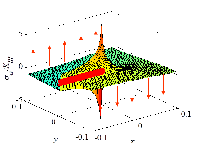
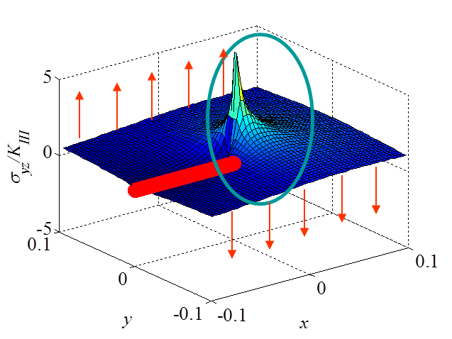
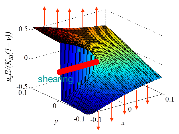
The asymptotic stress field (\ref{eq:stressAsympModeIII}) obtained for a Mode III loading is illustrated in Pictures II.27 and II.28. This last Picture II.28 represents the "yz"-stress component on which the stress concentration profile, which tends to infinity, is surrounded. The displacement field (\ref{eq:uModeIII}) is illustrated in Pictures II.29 were the crack shearing profile can be observed.
Summary on the asymptotic solution
For each mode of crack loading, see Pictures II.30, II.31 and II.32, we have found an asymptotic solution of the form
\begin{equation}\begin{cases} \mathbf{\sigma}^\text{mode i} = \frac{K_i}{\sqrt{2\pi r}} \mathbf{f}^\text{mode i}(\theta) \\ \mathbf{u}^\text{mode i} = K_i\sqrt{\frac{r}{2\pi}} \mathbf{g}^\text{mode i}(\theta) \end{cases},\label{eq:fandg}\end{equation}
where $\mathbf{f}$ and $\mathbf{g}$ are functions defined for each mode but independent of the loading and geometry (as long as we consider the asymptotic value), while the SIF $K_i$ depend on the geometry and loading conditions of the sample.
Since linear responses have been assumed, it is possible to use the principle of superposition, and $\mathbf{u}$ and $\mathbf{\sigma}$ can be added for:
- Different modes: $\mathbf{u} = \mathbf{u}_I + \mathbf{u}_{II}$ and $\mathbf{\sigma} = \mathbf{\sigma}_I + \mathbf{\sigma}_{II}$;
- Different loading conditions: $\mathbf{u} = \mathbf{u}^\text{a} + \mathbf{u}^\text{b}$ and $\mathbf{\sigma} = \mathbf{\sigma}^\text{a} + \mathbf{\sigma}^\text{b}$.
However one has to be careful that $\mathbf{f}$ and $\mathbf{g}$ are different for two different loading modes. So if $K_i$ can be added for different loading conditions $a$ and $b$ of the same mode $i$, i.e. $K_i = K_i^\text{a} + K_i^\text{b}$, the SIF of two different modes cannot be added, i.e. $K \neq K_I + K_{II}$.
The loading and geometry effects are thus fully reported to the value of the SIF. Irwin has thus the idea to consider the value of the SIF to detect the crack propagation. Indeed experiments have shown that for a given material, which obeys to the LEFM assumption, the crack propagates if the SIF reaches a threshold $K_C$ called the toughness of the material.
![]()