
SIF Computation >Numerical Approach (LEFM)
Extraction from the stress and displacement fields
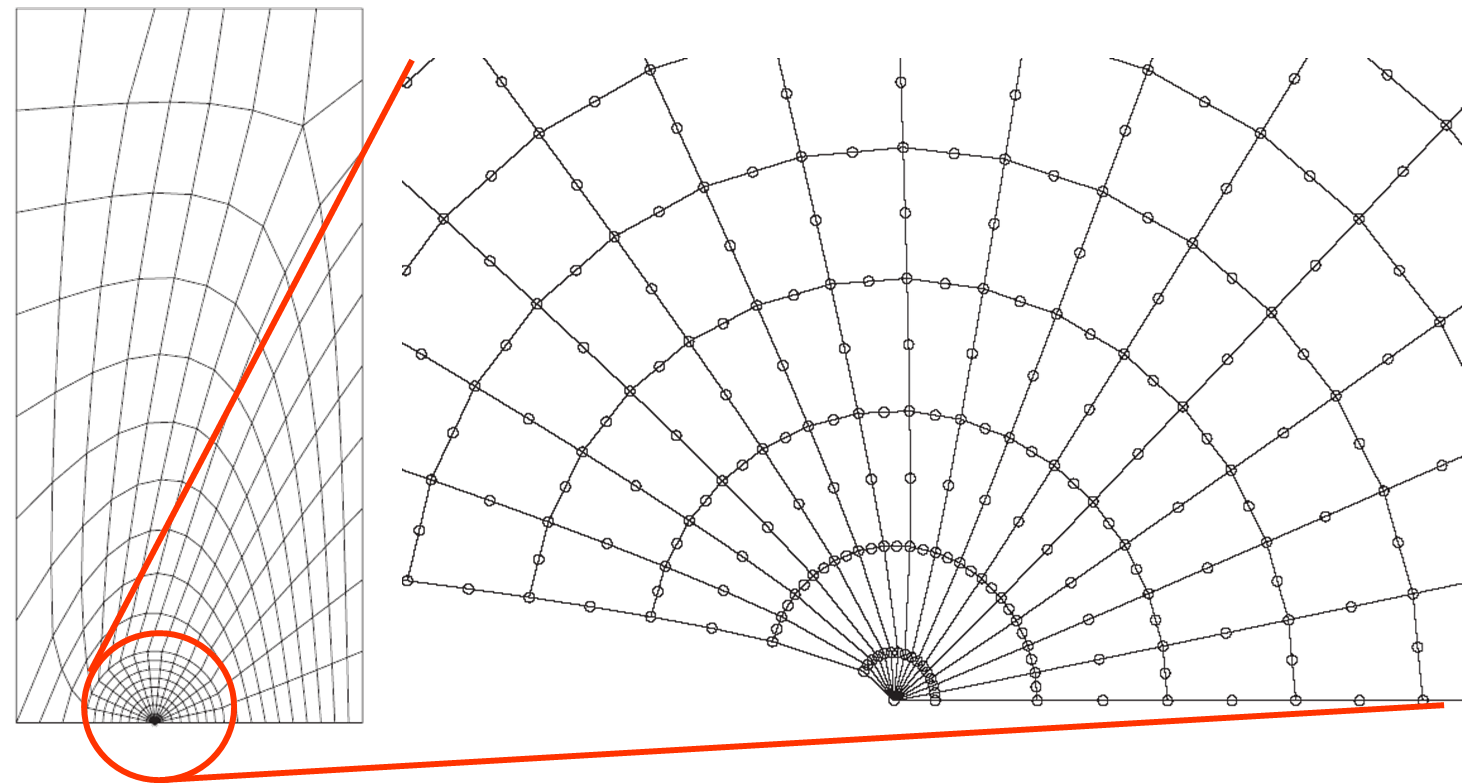
An increasingly popular way to solve a fracture mechanics problem is to consider a finite element model (FEM). In this section we consider FEMs which are conforming to the crack geometry, see Picture IV.15. On the one hand, the resolution of such a model provides the stress and displacement fields in the whole domain, and more particularly near the crack tip. On the other hand, the asymptotic solution provides the stress and displacement fields at crack tip in terms of the SIF:
\begin{equation} \begin{cases} \mathbf{\sigma}^{\text{mode}\, i} = \frac{K_i}{\sqrt{2\pi r}}f^{\text{mode}\, i}(\theta) \,;\\ u^{\text{mode}\, i} = K_{i}\sqrt{\frac{r}{2\pi}}g^{\text{mode}\, i}(\theta)\,.\end{cases}\label{eq:as}\end{equation}
Comparing the FE solution near the crack tip (and only there) to the asymptotic solution thus allows the SIFs to be identified.
Let us first consider the stress field ahead of the crack tip. Indeed, for mode I, $f(\theta=0)=1$ when considering $ \mathbf{\sigma}^{\text{mode}\, I}_{yy}$, in mode II, $f(\theta=0)=1$ when considering $ \mathbf{\sigma}^{\text{mode}\, II}_{xy}$, and in mode III, $f(\theta=0)=1$ when considering $ \mathbf{\sigma}^{\text{mode}\, III}_{yz}$. This means that the three SIFs can be evaluated from the stress field evolution ahead of the crack tip following
\begin{equation} \left( \begin{array}{c} K_I \\ K_{II} \\ K_{III} \end{array}\right) =\lim_{r\rightarrow 0} \sqrt{2\pi r} \left(\begin{array}{c} \mathbf{\sigma}_{yy}\left(r,0\right)\\ \mathbf{\sigma}_{xy}\left(r,0\right)\\ \mathbf{\sigma}_{zy}\left(r,0\right) \end{array}\right) \,.\end{equation}
The extrapolation of the stress field obtained by the FEM near the crack tip $\mathbf{\sigma}(r, \theta)$ can also be used to evaluate the SIFs. Indeed, for mode I, $g(\theta=\pm \pi)=\pm\frac{\left(\kappa+1\right)\left(\nu+1\right)}{E}$ when considering $ \mathbf{u}^{\text{mode}\, I}_{y}$, in mode II, $g(\theta=\pm \pi)=\pm\frac{\left(\kappa+1\right)\left(\nu+1\right)}{E}$ when considering $ \mathbf{u}^{\text{mode}\, II}_{x}$, and in mode III, $g(\theta=\pm \pi)=\pm\frac{1}{\mu}$ when considering $ \mathbf{u}^{\text{mode}\, III}_{z}$. This means that the three SIFs can be evaluated from the opening of the crack following
\begin{equation} \left( \begin{array}{c} \frac{4K_I}{E'} \\ \frac{4K_{II}}{E'} \\ \frac{K_{III}}{\mu} \end{array}\right) =\lim_{r\rightarrow 0} \sqrt{\frac{2\pi}{r}} \left(\begin{array}{c} u_y\left(r,\pi\right)\\ u_{x}\left(r,\pi\right)\\ u_{z}\left(r,\pi\right) \end{array}\right)\,, \end{equation}
where $E' = \frac{4E}{(1+\nu)(\kappa +1)} = \left\{\begin{array}{l l} E & P\mathbf{\sigma}\\ \frac{E}{1-\nu^2} &P \epsilon \end{array}\right.$ depends on the deformation state (through $\kappa$).
Advantages and drawbacks
The advantages of this method are:
- Its simplicity;
- It can be used with any FE software;
- Only post-processing is needed to determine the 3 SIFs;
- It can be used along a crack front in 3D;
- When using displacement correlation, the field is the primary solution so it is readily accessible.
The drawbacks of this method are
- The accuracy is strongly dependent on the mesh refinement;
- The required mesh refinement depends on the elements ability to capture the singularity at the crack tip (see next paragraph);
- It requires a modification of the mesh at each crack growth increment.
Barsoum elements
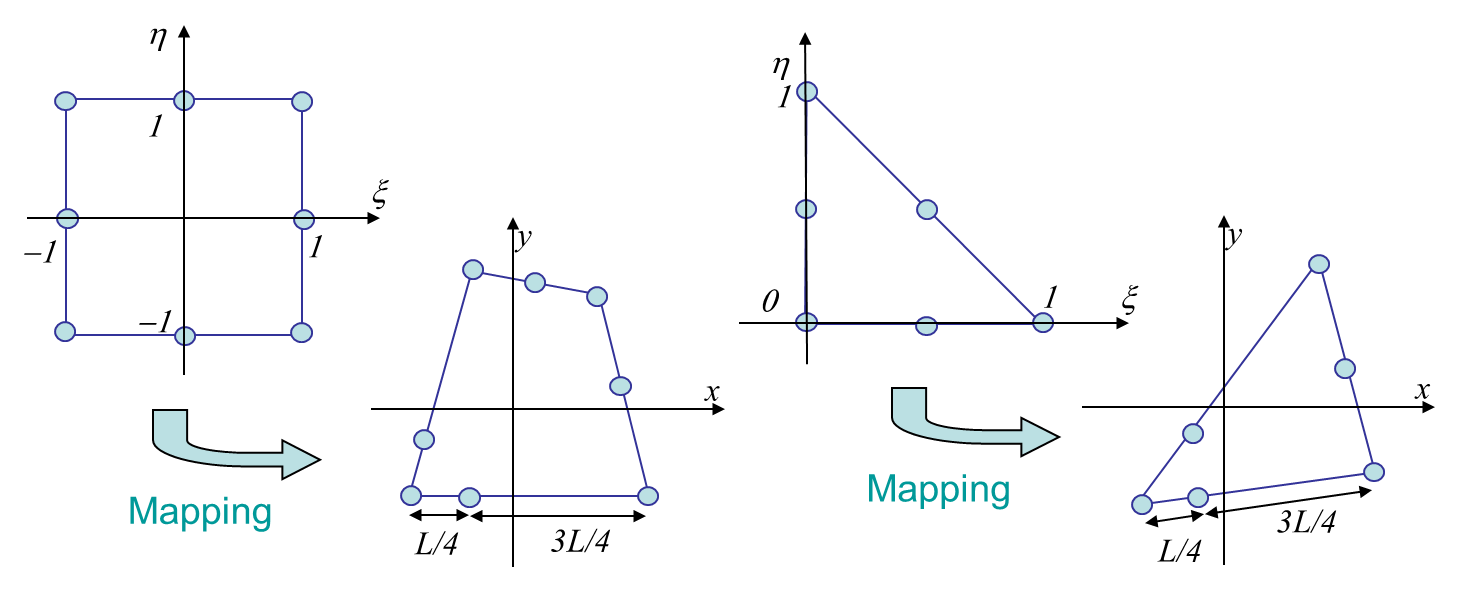
As shown in the previous section, the FEM can be used to predict the SIFs from the computed stress or displacement field. However, this method tries to capture the asymptotic behavior at the crack tip. Also, the asymptotic behavior is in $\sqrt{r}$, which is not well captured by usual FEs. For these reasons, the method requires a really fine mesh discretization at crack tip. It is thus interesting to modify the element so that the behavior in $\sqrt{r}$ can be captured. This can be achieved by enriching the elements (such as XFEM for LEFM, see later) or by using Barsoum elements (quarter-point elements). Quarter-point elements are quadratic elements with some mid-nodes located at a quarter of the edge, as shown in Picture IV.16.
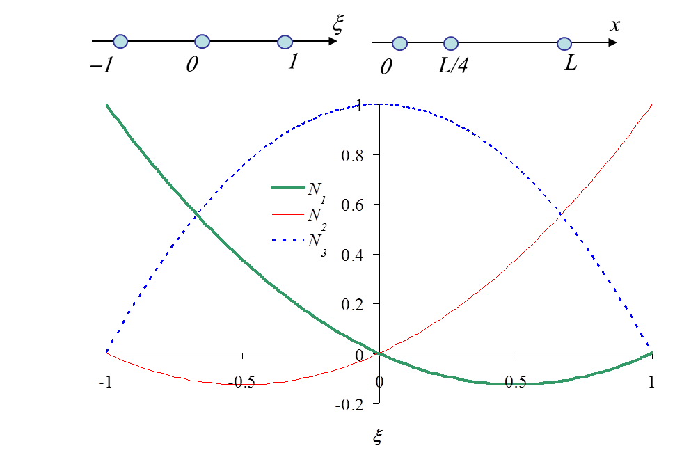
Indeed, such element allows the $\sqrt{r}$ trend to be captured as we will show it in the 1D case, see Picture IV.17. In 1D, the shape functions have the following expressions:
\begin{equation}
\left\{\begin{array}{r c l}
N_1 &=& \frac{\xi}{2}\left(\xi-1\right)\,;\\
N_2 &=& \frac{\xi}{2}\left(\xi+1\right)\,;\\
N_3 &=&\left(1-\xi^2\right)\,.\end{array}\right.
\end{equation}
The mapping of the 1D element, with the quarter point, see Picture IV.17, reads
\begin{equation} x\left(\xi\right) = N_i x_i = \frac{\xi L}{2}\left(\xi+1\right) +\frac{L}{4}\left(1-\xi^2\right)=\frac{L}{4}\left(1+\xi\right)^2\,.\end{equation}
Inverting this relation leads to
\begin{equation} \xi\left(x\right) =\sqrt{\frac{4x}{L}}-1 \,.\end{equation}
This allows expressing the strain from the displacement field following
\begin{equation} u = N_i\left(\xi\right) u_i \Longrightarrow \varepsilon=\partial_x u = \partial_\xi N_i\left(\xi\right) \partial_x \xi u_i=\frac{1}{\sqrt{Lx}}N_{i,\xi} u_i\,, \end{equation}
which shows that the method can capture a strain field in $1/\sqrt{r}$.
Practically the Barsoum elements are only introduced at the first row of finite elements at crack tip, as shown in Picture IV.15.
Global Energy & Compliance Methods
The extraction of the SIFs from the displacement or stress field of a finite element resolution is highly sensitive to the mesh resolution (especially when considering the stress field which is not a primary variable of the method). To avoid this problem it is better to consider global responses of the problem as the energy.
As a summary of the energetic approach, we have
- The energy release rate $G=J$ for crack growing straight ahead;
- The J-integral $J=\frac{K_I^2}{E'}+\frac{K_{II}^2}{E'}+\frac{K_{III}^2}{2\mu}$ in LEFM;
- For a prescribed loading: $G = \partial_A E_{int}|_Q$ in LEFM;
- For a prescribed displacement: $G =-\partial_A E_{int}|_a$.
Let us now consider two linear FE models of a structure, with the same loading (resp. displacement), but with two slightly different crack lengths $a$ and $a+\Delta a$. We can then compute numerically the energy release rate $G$ as
\begin{equation} G\simeq \pm \frac{E_\text{int}\left(a+\Delta a\right)-E_\text{int}\left(a\right)}{ t \Delta a}\,,\end{equation}
where $t$ is the thickness, and where the sign $+$ ($-$) holds for a prescribed loading (displacement). In LEFM, in terms of the structure compliance $C$ and of the general loading $Q$, this relation also reads
\begin{equation} G = Q^2\frac{C\left(a+\Delta a\right)-C\left(a\right)}{2\Delta a t}\,.\end{equation}
Advantages and drawbacks
The advantages of this method are:
- Its simplicity;
- It can be used with any FE software;
- Only post-processing is needed to determine the 3 SIFs;
- The lower mesh sensitive than for the correlation methods as a global variable is used.
The drawbacks of this method are
- 2 computations are required;
- Only 1 mode can be considered at a time as from $G$ only $\frac{K_I^2}{E'}+\frac{K_{II}^2}{E'}+\frac{K_{III}^2}{2\mu}$ can be deduced.
- In 3D, the SIF variation along the crack front cannot be determined.
Crack closure integral
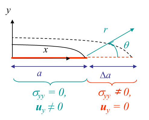
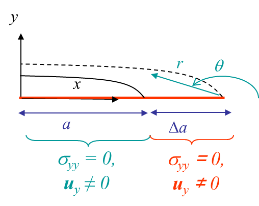
We have seen how to extract the SIFs from the energy release rate $G$. This last value was obtained from two FE simulations for which the crack size was increased by $\Delta a$. One alternative is to consider the crack closure integral between a configuration before the crack propagates and characterized by the stress field $\mathbf{\sigma}$ ahead of the crack tip, see Picture IV.18, and a configuration after the crack propagates and characterized by the crack opening $[\![\mathbf{u}]\!]$, see Picture IV.19. In linear elasticity, if the cracks grow straight ahead, we have
\begin{equation}G= \lim_{\Delta a\rightarrow 0} \frac{1}{t \Delta a}\int_0^{\Delta a}\frac{1}{2} \mathbf{\mathbf{\sigma}}_{iy}\left(r',\,0\right) [\![\Delta \mathbf{u}_i\left(\Delta a-r',\,\pi\right) ]\!] dr' \label{eq:GlinStraight1} \,.\end{equation}
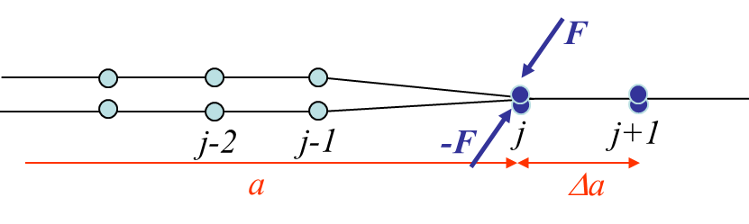
Equation (\ref{eq:GlinStraight1}) can be solved numerically when considering a FEM. Let us consider the FE mesh conforming with the crack surface: the crack tip corresponds to the node $j+1$, while nodes $j,\,j-1,\,j-2...$ lie on the crack lips and are duplicated (one on each lip), see Picture IV.20 and Picture IV.21. Two finite element simulations are now performed:
- For the first simulation the nodes $j$ on both lips are constrained to have the same position, see Picture IV.20. This corresponds to the configuration before crack propagation of Picture IV.18. The reaction force $\mathbf{F}$ required to constrain the two nodes is similar to the stress ahead of crack tip before the growth in (\ref{eq:GlinStraight1}) ;
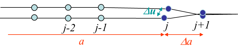
- For the second simulation the nodes $j$ on both lips are free to move apart, see Picture IV.21. This corresponds to the configuration after crack propagation of Picture IV.19. The nodes opening $\mathbf{\Delta u}$ is similar to the crack opening after the growth in (\ref{eq:GlinStraight1}).
Equation (\ref{eq:GlinStraight1}) can thus be approximated by
\begin{equation}G= \frac{\mathbf{F}\cdot\mathbf{\Delta u}}{2t \Delta a}\label{eq:GlinStraight1Num}\,. \end{equation}
The three SIFs can here be obtained from the components of the force $\mathbf{F}$ as each component corresponds to a loading mode:
\begin{equation}\begin{cases}\frac{K_I^2}{E'} = \frac{\mathbf{F}_y \mathbf{\Delta u}_y}{2t \Delta a}\,;\\ \frac{K_{II}^2}{E'} = \frac{\mathbf{F}_x \mathbf{\Delta u}_x}{2 t \Delta a}\,;\\ \frac{K_{III}^2}{2\mu} = \frac{\mathbf{F}_z \mathbf{\Delta u}_z}{2t \Delta a}\,.\end{cases}\end{equation}
Advantages and drawbacks
The advantages of this method are:
- It requires only post-processing.
The drawbacks of this method are:
- If the crack is not in a line of symmetry, the node displacements have to be constrained using Lagrange multipliers e.g.;
- 2 computations are needed (can be improved using modified nodal release).
The J-integral
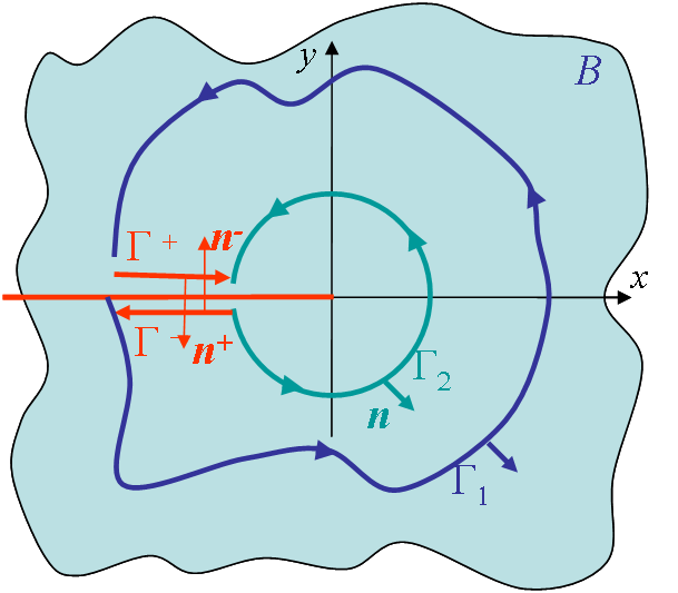
As a reminder, we can consider a cracked homogeneous material, with the crack parallel to the x-axis and with the contours $\Gamma_1$ and $\Gamma_2$ embedding the crack tip, see Picture IV.22. Thus the so-called J-integral, which is the energy that flows toward the crack tip, is defined as
\begin{equation} J = \int_{\Gamma_1} \left[U\left(\mathbf{\varepsilon}\right) \mathbf{n}_x - \mathbf{\mathbf{u}}_{,x} \cdot \mathbf{T}\right] dl = \int_ {\Gamma_2} \left[U\left(\mathbf{\varepsilon}\right) \mathbf{n}_x - \mathbf{\mathbf{u}}_{,x} \cdot \mathbf{T}\right] dl.\label{eq:J} \end{equation}
As it can be deduced from (\ref{eq:J}), this integral
- Is path independent (as long as the contour embeds the crack tip);
- Does not request linearity of the material (only the existence of an internal potential has been assumed);
- Does not depend on the subsequent crack growth direction.
In linear elasticity, we have also shown that
\begin{equation}J=\frac{K^2_I}{E'}+\frac{K^2_{II}}{E'}+\frac{K^2_{III}}{2\mu}\label{eq:JSIF}\end{equation}
Computing the J-integral is thus a way to evaluate the SIFs. Note that is the crack grows straight ahead, once also has $G=J$.
Direct computation of the J-integral
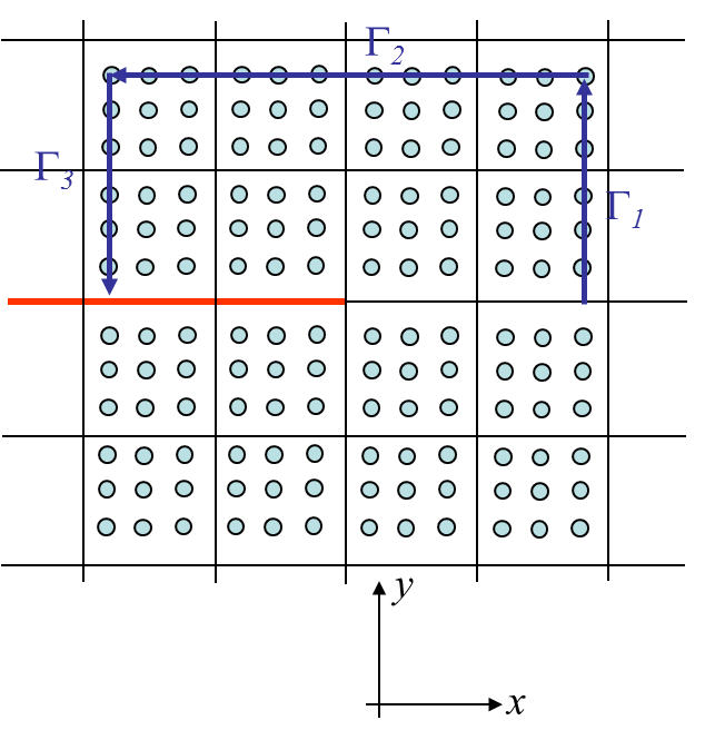
In order to compute (\ref{eq:J}) during a FE resolution, the simplest method is to create a contour passing through the Gauss points, see Picture IV.23. The J-integral can thus be computed from the fields at the Gauss points:
\begin{equation}\begin{array}{ll} \frac{J}{2} &=& \int_{\Gamma_1} \left[\frac{\mathbf{\mathbf{\sigma}}_{ij}\varepsilon_{ij}}{2} -\mathbf{\mathbf{\sigma}}_{xi}\mathbf{u}_{i,x}\right] dl -\int_{\Gamma_2}\left[ \mathbf{\mathbf{\sigma}}_{yi}\mathbf{u}_{i,x}\right] dl + \\&&\int_{\Gamma_3}\left[-\frac{\mathbf{\mathbf{\sigma}}_{ij}\epsilon_{ij}}{2} +\mathbf{\mathbf{\sigma}}_{xi}\mathbf{u}_{i,x}\right] dl\,, \end{array} \end{equation}
where $dl=dy$ on $\Gamma_,$, $dl=-dx$ on $\gamma_2$ and $dl =-dy$ on $\Gamma_3$. The difficulty of this method is to generate a contour passing through all the Gauss points of interest, particularly when considering unstructured meshes.
J-integral by domain integration
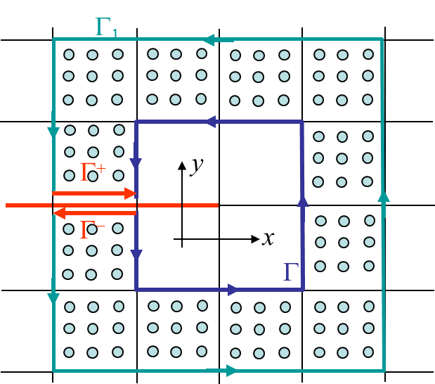
In order to avoid the difficulties linked to the definition of a Gauss-points contour, one alternative is to transform the contour integral (\ref{eq:J}) into a domain integral. To this end we can define a closed contour: $C=\Gamma_1 +\Gamma^-+\Gamma^+-\Gamma$, whose interior is called $D$, see Picture IV.24. We can then define a field $q(x,y)$ such that $q=1$ on $\Gamma$ and $q=0$ on $\Gamma_1$. Moreover, as $\mathbf{n}_x=\mathbf{T}=0$ on $\Gamma^-+\Gamma^+-$, the J-integral (\ref{eq:J}) can be rewritten
\begin{equation} \begin{array}{ll} J &=& \int_{\Gamma} \left[U\left(\mathbf{\varepsilon}\right) \mathbf{n}_x q - \mathbf{u}_{,x} \cdot \mathbf{T} q \right] dl -\\ && \int_{\Gamma_1} \left[U\left(\mathbf{\varepsilon}\right) \mathbf{n}_x q - \mathbf{u}_{,x} \cdot \mathbf{T} q \right] dl\,. \label{eq:Jdom1}\end{array}\end{equation}
As the crack is stress free, one has
\begin{equation} \int_{\Gamma^\pm} \left[U\left(\mathbf{\varepsilon}\right) \mathbf{n}_x q - \mathbf{u}_{,x} \cdot \mathbf{T} q \right] dl=0\,, \end{equation}
and (\ref{eq:Jdom1}) becomes
\begin{equation} J = -\int_{C} \left[U\left(\mathbf{\varepsilon}\right) \mathbf{n}_x q - \mathbf{u}_{,x} \cdot \mathbf{T} q \right] dl\,. \end{equation}
As the contour $C$ is closed and as $\mathbf{T}=\mathbf{\sigma}\cdot\mathbf{n}$, we can use the divergence theorem, and this last equation is rewritten
\begin{equation} J = \int_{D} \left\{ \nabla\cdot\left[\mathbf{u}_{,x} \cdot \mathbf{\sigma}\, q \right]- \left[U\left(\mathbf{\varepsilon}\right) q\right]_{,x} \right\} dA \,.\end{equation}
In the general non-linear conservative case we have $U_{,x}=\partial U/\partial \mathbf{\varepsilon} :\mathbf{\varepsilon}_{,x}= \mathbf{\sigma}:\mathbf{\varepsilon}_{,x}$ and the linear momentum equation, in the absence of body and inertial forces reads $\mathbf{\sigma}_{ij,j}=0$. Substituting these relations in the last result leads to
\begin{equation} J = \int_{D} \left\{ \mathbf{\sigma}_{ij}\left[\mathbf{u}_{i,x} q \right]_{,j}-\mathbf{u}_{i,jx}\mathbf{\sigma}_{ij}q- U q_{,x} \right\} dA\,, \end{equation}
or again
\begin{equation} J =\int_{D} \left[ \mathbf{\sigma}_{ij}\mathbf{u}_{i,x} q_{,j} - U q_{,x} \right] dA\,.\label{eq:Jdom} \end{equation}
We can thus compute from a FE resolution the J-integral using (\ref{eq:Jdom}) by defining a contour of elements, instead of a contour of Gauss points. Practically
- The field $q$ is discretized using the same shape functions than the displacements;
- As this integral is valid for any annular region around the crack tip, as long as the crack lips are straight, we can chose the annular region far enough from the crack tip.
Advantages and drawbacks
The advantages of this method are:
- Its accuracy (especially using domain integration);
- It does not require Barsoum elements.
The drawbacks of this method are:
- Only one SIF related to a mode can be evaluated at once as $J$ involves the three SIFs, see (\ref{eq:JSIF});
- It requires either to modify the FE code in order to have an easy post processing, or
- The post-processing is difficult when using a standard FE software(requires to dump all the Gauss points variables).
Extraction of individual SIFs
Because of the accuracy of the J-integral method, efforts have been put to develop a method so that the three SIFs can be extracted separatly from the J-integral. To this end we need to consider three problems:
- First we need to compute $J$ for the solution $\mathbf{u}$ of the considered problem, leading to
\begin{equation}J = \int_{\Gamma} \left[U\left(\mathbf{\varepsilon}\right) \mathbf{n}_x - \mathbf{u}_{,x} \cdot \mathbf{T}\right] dl =\frac{K^2_I}{E'}+\frac{K^2_{II}}{E'}+\frac{K^2_{III}}{2\mu} \,, \label{eq:J1} \end{equation}
where $K_I$, $K_{II}$, and $K_{III}$ are the sought values. - In a second step, we compute the J-integral for another solution field $\mathbf{u}^{aux}$ that needs to be specialized. This yields the so-called auxiliary J-value:
\begin{equation} J^{aux}= \int_{\Gamma} \left[U\left(\mathbf{\varepsilon}^{aux}\right) \mathbf{n}_x - \mathbf{u}_{,x}^{aux} \cdot \mathbf{T}\left(\mathbf{u}^{aux}\right)\right] dl = \frac{{K^{aux}_I}^2}{E'}+\frac{{K^{aux}_{II}}^2}{E'}+ \frac{{K^{aux}_{III}}^2}{2\mu}\label{eq:J2} \,.\end{equation} - Then we compute $J$ for a third problem which is the superposition of the first two ones, so that the displacement field becomes $\mathbf{u}+\mathbf{u}^{aux}$ in linear elasticity. The resulting J-integral reads
\begin{equation} J^s= \int_{\Gamma} \left[U\left(\mathbf{\varepsilon}+\mathbf{\varepsilon}^{aux}\right) \mathbf{n}_x - \left(\mathbf{u}_{,x}+\mathbf{u}^{aux}_{,x}\right) \cdot \mathbf{T}\left(\mathbf{u}+\mathbf{u}^{aux}\right)\right] dl \label{eqJs}\,. \end{equation}
The relation between the different values of $J$ can be deduced from these two relations:
\begin{equation} \begin{cases} U\left(\mathbf{\varepsilon}+\mathbf{\varepsilon}^{aux}\right) =\frac{1}{2}\left(\nabla\mathbf{u}+\nabla\mathbf{u}^{aux}\right):\mathcal{H}:\left(\nabla\mathbf{u}+\nabla\mathbf{u}^{aux}\right)= U\left(\mathbf{\varepsilon}\right)+U\left(\mathbf{\varepsilon}^{aux}\right)+\nabla\mathbf{u}:\mathcal{H}:\nabla\mathbf{u}^{aux}\,;\\ \left(\mathbf{u}_{,x}+\mathbf{u}^{aux}_{,x}\right) \cdot \mathbf{T}\left(\mathbf{u}+\mathbf{u}^{aux}\right) =\mathbf{u}_{,x}\cdot\mathbf{T}\left(\mathbf{u}\right) + \mathbf{u}_{,x}^{aux}\cdot\mathbf{T}\left(\mathbf{u}^{aux}\right) + \mathbf{u}_{,x}\cdot\mathbf{T}\left(\mathbf{u}^{aux}\right) +\mathbf{u}_{,x}^{aux}\cdot\mathbf{T}\left(\mathbf{u}\right) \,. \end{cases} \end{equation}
Indeed, using these identities, equation (\ref{eqJs}) can be rewritten as the interaction integral:
\begin{equation} J^s-J-J^{aux} = \int_{\Gamma} \left[\nabla\mathbf{u}:\mathcal{H}:\nabla\mathbf{u}^{aux} \mathbf{n}_x - \mathbf{u}_{,x}\cdot\mathbf{T}\left(\mathbf{u}^{aux}\right) -\mathbf{u}_{,x}^{aux}\cdot\mathbf{T}\left(\mathbf{u}\right) \right] dl\,.\label{eq:interJ}\end{equation}
In linear elasticity, we can use the asymptotic solution (\ref{eq:as}) to express the displacement and the stress fields in terms of the stress intensity factors
\begin{equation} \left\{\begin{array}{r c l} \sigma &=& \sum_{i =I}^{III}\frac{K_i}{\sqrt{2\pi r}} \mathbf{f}^{\text{mode i}}\left(\theta\right)\,;\\ \sigma\left(\mathbf{u}^{aux}\right) &=&\sum_{i =I}^{III} \frac{K_i^{aux}}{\sqrt{2\pi r}} \mathbf{f}^{\text{mode i}}\left(\theta\right)\,; \\ \mathbf{u} &=&\sum_{i =I}^{III} K_i\sqrt{\frac{r}{2\pi}} \mathbf{g}^{\text{mode i}}\left(\theta\right)\,;\\ \mathbf{u}^{aux} &=& \sum_{i =I}^{III} K_i^{aux}\sqrt{\frac{r}{2\pi}} \mathbf{g}^{\text{mode i}}\left(\theta\right)\,.\end{array}\right. \end{equation}
The direct substitution of these relations into the terms of the interaction integral (\ref{eq:interJ}) leads to
\begin{equation}\begin{cases} \nabla\mathbf{u}:\mathcal{H}:\nabla\mathbf{u}^{aux}& =& \sum_i\sum_j K_i K_j^{aux} \nabla \frac{\sqrt{r}\mathbf{g}^{\text{mode i}}}{\sqrt{2\pi}}:\mathcal{H}:\nabla \frac{\sqrt{r}\mathbf{g}^{\text{mode j}}}{\sqrt{2\pi}}\,;\\ \mathbf{u}_{,x}\cdot\sigma\left(\mathbf{u}^{aux}\right) +\mathbf{u}_{,x}^{aux}\cdot\sigma \left(\mathbf{u}\right) &=& \sum_i\sum_j\left[ K_i K_j^{aux} \partial_x \frac{\sqrt{r} \mathbf{g}^{\text{mode i}}}{\sqrt{2\pi}}\cdot\frac{\mathbf{f}^{\text{mode j}}}{\sqrt{2\pi r}}\right.\\&&\left. + K_j K_i^{aux} \partial_x \frac{\sqrt{r} \mathbf{g}^{\text{mode i}}}{\sqrt{2\pi}} \cdot\frac{\mathbf{f}^{\text{mode j}}}{\sqrt{2\pi r}}\right]\,.\end{cases} \end{equation}
Proceeding as to obtain the original relationship between $J$ and the SIFs, the direct substitution of the functions $f$ and $g$ by their expressions in these last two identities allows rewriting the interaction integral (\ref{eq:interJ}) as
\begin{equation} \frac{J^s-J-J^{aux}}{2} =\frac{K_IK^{aux}_I}{E'}+\frac{K_{II}K^{aux}_{ii}}{E'}+\frac{K_{III}K_{III}^{aux}}{2\mu}\,. \label{eq:Jinteraction}\end{equation}
It is thus clear that to evaluate $K_i$, $i=1,\,2\,,3$, $\mathbf{u}^{aux}$ should be chosen such that only $K_i^{aux}\neq 0$.
As said the extraction of one SIF requires two more finite element resolutions (one with $\mathbf{u}^{aux}$ and one with $\mathbf{u}+\mathbf{u}^{aux}$) which make the computation of the SIFs quite expensive.
![]()