
Asymptotic Solution > The Airy function for a cracked plate
Remember that in the previous section we found that 2D problems with a linear elastic material law can be stated as finding $\Phi$ so that the boundary conditions and
\begin{equation} \nabla^2\nabla^2 \Phi =0 \label{eq:biharmonic},\end{equation}
are satisfied. The problem is thus to find the suitable $\Phi$.
Complex variables and functions
\begin{equation}\begin{cases} \mathbf{\sigma}_{zz} = 0 \text{ or } \mathbf{\varepsilon}_{zz} = 0 \\ \mathbf{\sigma}_{yy}(\theta \pm \pi) = 0 \\ \mathbf{\sigma}_{xy}(\theta \pm \pi) = 0 \\ \mathbf{u}_x (\theta) = \mathbf{u}_x (-\theta) \\ \mathbf{u}_y (\theta) = -\mathbf{u}_y (-\theta) \end{cases},\label{eq:bcModeI}\end{equation} |
\begin{equation}\begin{cases} \mathbf{\sigma}_{zz} = 0\text{ or } \mathbf{\varepsilon}_{zz} = 0 \\ \mathbf{\sigma}_{yy}(\theta \pm \pi) = 0 \\ \mathbf{\sigma}_{xy}(\theta \pm \pi) = 0 \\ \mathbf{u}_x (\theta) = -\mathbf{u}_x (-\theta) \\ \mathbf{u}_y (\theta) = \mathbf{u}_y (-\theta) \end{cases},\label{eq:bcModeII}\end{equation} |
|
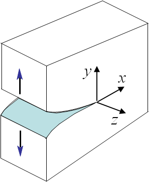
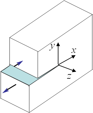
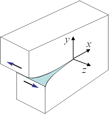
As shown in the previous problem of a plate with an elliptical hole, there is a singularity if $b\rightarrow 0$. We will then have to modify the resolution method when considering a plate with a crack. Irwin has solved this problem for three different loading modes. There are two modes loading the crack in its plane, the Mode I also called opening mode as it tends to open the crack lips, see Picture II.8, and the Mode II also called sliding mode as it tends to make the two crack lips slide on each other, see Picture II.9. The Mode III, also called shearing mode, loads the crack out of its plane, see Picture II.10. To do so the polar coordinates linked to the crack tip will be used, see Picture II.11. The only things that differentiate the three modes are the boundary conditions of the problem, which can directly be written in terms of the polar coordinates as (\ref{eq:bcModeI}-\ref{eq:bcModeIII}). Once the boundary conditions are known, it is possible to solve the problem.
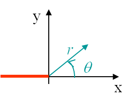
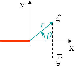
Because of the shape of the crack, there will be a discontinuity in the solution at the crack location. It is thus convenient to solve the problem in terms of a complex variable $\zeta=x+iy=r \mathrm{e}^{i\theta}$ using axes linked to the crack tip, see Picture II.12. Let us now remind the concept of a complex function
\begin{equation} z\left(\zeta\right)= \alpha\left(x,\,y\right)+i\beta\left(x,\,y\right)\label{eq:complexz},\end{equation}
constructed from $\alpha$ and $\beta$ two real functions so that $\alpha=\mathcal{R}\left(z\left(\zeta\right)\right)$ and $\beta=\mathcal{I}\left(z\left(\zeta\right)\right)$. Assuming $z$ is differentiable, i.e. it is analytic, then one can prove that
\begin{equation} z'\left(\zeta\right) = \partial_x z=-i\partial_y z \label{eq:analyticz}.\end{equation}
Using this last result leads directly to the Cauchy-Riemann relations
\begin{equation}\begin{cases} &\partial_x z = \alpha_{,x} +i \beta_{,x} = -i\partial_y z = -i \alpha_{,y} + \beta_{,y} \\& \iff \alpha_{,x} = \beta_{,y} \text{ and } \alpha_{,y} = - \beta_{,x}\end{cases}\label{eq:cauchyRiemann1}.\end{equation}
Differentiating these last relations yields
\begin{equation}\begin{cases} &\alpha_{,xx} = \beta_{,xy} = - \alpha_{,yy} \text{ and } & \beta_{,xx} =- \alpha_{,xy} = - \beta_{,yy}\\ & \iff \nabla^2 \alpha = \nabla^2 \beta= 0 \end{cases}.\label{eq:cauchyRiemann}\end{equation}
This means that if $z$ is analytic, then its real and imaginary function parts (both of which are real functions) satisfy the Laplace equation. Similarly, if a real function satisfies the Laplace equation, then it is the real or imaginary function part of an analytic function $z$.
Solution of the bi-harmonic equation
In order to solve (\ref{eq:biharmonic}), we now need to consider a change of variables to use the complex variable $\zeta$ defined on Picture II.12. As the original function $\Phi$ depends on two original variables $x$ and $y$, we also need two new variables. To easily express $x$ and $y$ in terms of the two new variables we select $\zeta$ and its conjugated value $\bar{\zeta}$, as
\begin{equation}\begin{cases} x = \frac{\zeta +\bar{\zeta}}{2}\\ y = i \frac{\bar{\zeta} -\zeta}{2}\end{cases},\label{eq:chgeComplex}\end{equation}
and we have
\begin{equation} \Phi(x,y) = \Phi(\zeta,\, \bar{\zeta}) \end{equation}
Let us define $\Psi$ such that
\begin{equation} \nabla^2\Phi\left(\zeta,\,\bar{\zeta}\right) = \Psi\left(\zeta,\,\bar{\zeta}\right)\,\label{eq:Psi2} \end{equation}
To express the Laplacian of $\Phi$ in terms of the complex variables, we need to compute the derivatives of the Airy function using the change of variables (\ref{eq:chgeComplex}):
\begin{equation}\begin{cases} \Phi_{,xx} = & \partial_x\left(\Phi_{,\zeta} + \Phi_{,\bar{\zeta}} \right) = \Phi_{,\zeta\zeta} + 2\Phi_{,\zeta\bar{\zeta}}+ \Phi_{,\bar{\zeta}\bar{\zeta}} \\ \Phi_{,yy} = & \partial_y\left(i \Phi_{,\zeta} - i \Phi_{,\bar{\zeta}} \right) = -\Phi_{,\zeta\zeta} + 2\Phi_{,\zeta\bar{\zeta}}- \Phi_{,\bar{\zeta}\bar{\zeta}} \end{cases},\label{eq:derviPhi}\end{equation}
and we finally have
\begin{equation} \Psi = \nabla^2\Phi = \Phi_{,xx} + \Phi_{,yy} = 4\Phi_{,\zeta\bar{\zeta}}.\label{eq:Psi}\end{equation}
Now the bi-harmonic equation (\ref{eq:biharmonic}) is rewritten
\begin{equation} \nabla^2\nabla^2\Phi\left(\zeta,\,\bar{\zeta}\right) = \nabla^2\Psi\left(\zeta,\,\bar{\zeta}\right)=0. \end{equation}
Since $\Psi$ satisfies the Laplace equation (\ref{eq:cauchyRiemann}), it is the real part of a function $z(\zeta)$ and we have from (\ref{eq:Psi})
\begin{equation} 4\Phi_{,\zeta\bar{\zeta}}=\Psi\left(\zeta,\,\bar{\zeta}\right) = \mathcal{R}z=\frac{z+\bar{z}}{2} \label{eq:system}\end{equation}
with $\bar{z} = z(\bar{\zeta})$, a function of $\bar{\zeta}$ only. The equation $4\Phi_{,\zeta\bar{\zeta}}=\frac{z+\bar{z}}{2}$ is now integrated with respect to $\zeta$ and to $\bar{\zeta}$ -do not forget during the integration with respect to one variable to add a function which is constant in terms of that variable, but not in terms of the other one. Let $4\Omega'(\zeta) = z(\zeta)$ and $\omega(\zeta)$ be unknown functions, then
\begin{equation} \Phi = \frac{\bar{\zeta}\Omega+\zeta\bar{\Omega} + \omega + \bar{\omega}}{2} \label{eq:PhiCrack},\end{equation}
which satisfies (\ref{eq:system}) as
\begin{equation} 4 \Phi_{,\zeta\bar{\zeta}} = 2\left(\Omega' + \bar{\Omega}'\right)=\frac{z+\bar{z}}{2} \end{equation}
Note well that $\bar{\Omega} = \Omega(\bar{\zeta})$ and $\bar{\omega} = \omega(\bar{\zeta})$ are functions of $\bar{\zeta}$ only.
What needs to be understood at this level is the following. If one can find two functions $\Omega(\zeta)$ and $\omega(\zeta)$ so that the BCs of the problem are satisfied, then we have solved the problem of a cracked plate. Indeed for any expressions of $\Omega(\zeta)$ and $\omega(\zeta)$, the Airy function (\ref{eq:PhiCrack}) automatically satisfies the bi-harmonic equation, and thus the linear momentum and elastic constitutive equations. So we "just" have to find the proper functions $\Omega(\zeta)$ and $\omega(\zeta)$ which satisfy the BCs. To do so we need to express the stress tensor and the displacement field from these functions.
Stress components in terms of the unknown functions
The stress tensor can be obtained from the derivative of the Airy function as given from the expression in the Cartesian coordinates. We will need to apply the change of variables, but before we will express the derivatives of (\ref{eq:PhiCrack}) with respect to the new variables $\zeta$ and $\bar{\zeta}$. As $\Omega(\zeta)$ and $\omega(\zeta)$ are function of $\zeta$ only, and as $\bar{\Omega} = \Omega(\bar{\zeta})$ and $\bar{\omega} = \omega(\bar{\zeta})$ are functions of $\bar{\zeta}$ only, one has
\begin{equation}\begin{cases} \Phi_{,\zeta\zeta} =& \frac{\bar{\zeta}\Omega''+\omega''}{2}\\\Phi_{,\zeta\bar{\zeta}} =& \frac{\Omega'+\bar{\Omega}'}{2}\\\Phi_{,\bar{\zeta}\bar{\zeta}} =& \frac{\zeta\bar{\Omega}''+\bar{\omega}''}{2} \end{cases}\label{eq:DerivPhiCrack}.\end{equation}
Now, starting from stress the expression in Cartesian coordinates, and using (\ref{eq:DerivPhiCrack}), the change of variables (\ref{eq:chgeComplex}) leads to
\begin{equation}\begin{cases} \mathbf{\sigma}_{xx} = & \Phi_{,yy} =-\Phi_{,\zeta\zeta} + 2\Phi_{,\zeta\bar{\zeta}}- \Phi_{,\bar{\zeta}\bar{\zeta}}=\Omega' +\bar{\Omega}' -\frac{\bar{\zeta}\Omega''+\zeta\bar{\Omega}'' + \omega'' + \bar{\omega}''}{2}\\ \mathbf{\sigma}_{yy} = & \Phi_{,xx}=\Phi_{,\zeta\zeta} + 2\Phi_{,\zeta\bar{\zeta}}+ \Phi_{,\bar{\zeta}\bar{\zeta}}=\Omega' +\bar{\Omega}' +\frac{\bar{\zeta}\Omega''+\zeta\bar{\Omega}'' + \omega'' + \bar{\omega}''}{2} \\ \mathbf{\sigma}_{xy} = & -\Phi_{,xy}=-i\Phi_{,\zeta\zeta} +i \Phi_{,\bar{\zeta}\bar{\zeta}}=i \frac{\zeta\bar{\Omega}''-\bar{\zeta}\Omega'' + \bar{\omega}''- \omega'' }{2}\end{cases} \label{eq:stressAiry}. \end{equation}
Displacement field in terms of the unknown functions
How can the displacements be written in terms of the two functions $\Omega(\zeta)$ and $\omega(\zeta)$? We know that the displacement field is the integration of the strain field, which can be related to the stress tensor in terms of the Hooke law. To introduce the complex variables, we define $\mathbf{u}\left(\zeta,\,\bar{\zeta}\right) = \mathbf{u}_x\left(x,\,y\right) + i \mathbf{u}_y \left(x,\,y\right)$. The strain field can be introduced in this equation by simple derivation
\begin{equation}\begin{cases}\mathbf{u}_{,\bar{\zeta}} = \left(\mathbf{u}_{x,x}+i\mathbf{u}_{y,x}\right)\partial_{\bar{\zeta}}x
+\left(\mathbf{u}_{x,y}+i\mathbf{u}_{y,y}\right)\partial_{\bar{\zeta}}y = \frac{1}{2}\left(\mathbf{u}_{x,x}+i\mathbf{u}_{y,x}+i\mathbf{u}_{x,y}-\mathbf{u}_{y,y}\right)\\ \iff \mathbf{u}_{,\bar{\zeta}}=\frac{1}{2}\left(\mathbf{\varepsilon}_{xx}-\mathbf{\varepsilon}_{yy}\right) +i\mathbf{\varepsilon}_{xy}\end{cases}.\label{eq:dU}\end{equation}
Introducing Hooke's law expressed in plane stress (P-$\sigma$) or plane strain (P-$\varepsilon$) states, and using (\ref{eq:stressAiry}) leads for both cases to
\begin{equation} \mathbf{u}_{,\bar{\zeta}} =
\frac{1+\nu}{2E}\left(\mathbf{\sigma}_{xx}-\mathbf{\sigma}_{yy}+2i\mathbf{\sigma}_{xy}\right) = -\frac{1+\nu}{E}\left(\zeta\bar{\Omega}''+\bar{\omega}''\right)\label{eq:derivU},
\end{equation}
which can be integrated with respect to $\bar{\zeta}$ as
\begin{equation} \mathbf{u} = -\frac{1+\nu}{E}\left(\zeta\bar{\Omega}'+\bar{\omega}' + \mu \left(\zeta\right)\right), \label{eq:uTmpAiry} \end{equation}
where the function $\mu\left(\zeta\right)$ is constant with respect to $\bar{\zeta}$ and should be defined to satisfy the P-$\sigma$ or P-$\varepsilon$ states.
Plane stress state
On the one hand, from the definition of $\mathbf{u}$, one has
\begin{equation}\begin{cases}
\mathbf{u}_{,\zeta} &=
\left(\mathbf{u}_{x,x}+i\mathbf{u}_{y,x}\right)\partial_{\zeta}x
+\left(\mathbf{u}_{x,y}+i\mathbf{u}_{y,y}\right)\partial_{\zeta}y =\frac{1}{2}\left(\mathbf{u}_{x,x}+i\mathbf{u}_{y,x}-i\mathbf{u}_{x,y}+\mathbf{u}_{y,y}\right)\\
\bar{\mathbf{u}}_{,\bar{\zeta}} &= \left(\mathbf{u}_{x,x}-i\mathbf{u}_{y,x}\right)\partial_{\bar{\zeta}}x
+\left(\mathbf{u}_{x,y}-i\mathbf{u}_{y,y}\right)\partial_{\bar{\zeta}}y =
\frac{1}{2}\left(\mathbf{u}_{x,x}-i\mathbf{u}_{y,x}+i\mathbf{u}_{x,y}+\mathbf{u}_{y,y}\right)\end{cases}\label{eq:dU1},\end{equation}
which implies
\begin{equation}
\mathbf{u}_{,\zeta}+\bar{\mathbf{u}}_{,\bar{\zeta}} =
\mathbf{u}_{x,x}+\mathbf{u}_{yy}=\mathbf{\varepsilon}_{xx}+\mathbf{\varepsilon}_{yy}=\mathbf{\varepsilon}_{\gamma\gamma}.\label{eq:dU2}
\end{equation}
On the other hand, starting from (\ref{eq:uAiry}), one has
\begin{equation} \mathbf{u}_{,\zeta}+\bar{\mathbf{u}}_{,\bar{\zeta}} =-\frac{1+\nu}{E}\left(\bar{\Omega}'+ \mu'+\Omega'+ \bar{\mu}'\right).\label{eq:dU3} \end{equation}
Combining (\ref{eq:dU2}) and (\ref{eq:dU3}) leads to
\begin{equation} \mathbf{\varepsilon}_{\gamma\gamma} =-\frac{1+\nu}{E}\left(\bar{\Omega}'+ \mu'+\Omega'+ \bar{\mu}'\right).\label{eq:traceEps} \end{equation}
The Hooke's law expressed in plane stress (P-$\sigma$) can be rewritten using (\ref{eq:stressAiry}), and becomes
\begin{equation}
\mathbf{\varepsilon}_{\gamma\gamma}
=\frac{1-\nu}{E}\mathbf{\sigma}_{\gamma\gamma} = \frac{2\left(1-\nu\right)}{E}\left(\Omega'+\bar{\Omega}'\right)
.\label{eq:traceEpsPstress}
\end{equation}
Comparing this last equation with (\ref{eq:traceEps}) gives the expression of the missing function
\begin{equation} \mu\left(\zeta\right) = -\frac{3-\nu}{1+\nu}\Omega= - \kappa \Omega\left(\zeta\right),
\end{equation}
with $
\kappa =\frac{3-\nu}{1+\nu}$.
Plane strain state
We can proceed as for the P-$\sigma$ state up to (\ref{eq:traceEps}). At this point, the Hooke's law expressed in plane strain (P-$\varepsilon$) can be rewritten using (\ref{eq:stressAiry}), and becomes
\begin{equation}\mathbf{\varepsilon}_{\gamma\gamma} =\frac{\left(1+\nu\right)\left(1-2\nu\right)}{E}\mathbf{\sigma}_{\gamma\gamma}=
\frac{2\left(1+\nu\right)\left(1-2\nu\right)}{E}\left(\Omega'+\bar{\Omega}'\right).\label{eq:traceEpsPstrain}
\end{equation}
Comparing this last equation with (\ref{eq:traceEps}) gives the expression of the missing function
\begin{equation} \mu\left(\zeta\right) = -\left(3-4\nu\right)\Omega= - \kappa \Omega\left(\zeta\right), \end{equation}
with $ \kappa =3-4\nu$.
Summary of plane stress and strain states
For both cases we found the expression of the missing function as being
\begin{equation} \mu\left(\zeta\right) - \kappa \Omega\left(\zeta\right).\label{eq:mu} \end{equation}
This means (\ref{eq:uTmpAiry}) can be rewritten
\begin{equation} \mathbf{u}\left(\zeta,\,\bar{\zeta}\right) = -\frac{1+\nu}{E}\left(\zeta\bar{\Omega}'\left(\bar{\zeta}\right)+\bar{\omega}'\left(\bar{\zeta}\right) -\kappa\Omega\left(\zeta\right)\right),\label{eq:uAiry} \end{equation}
with
\begin{equation}\kappa = \begin{cases}\frac{3-\nu}{1+\nu} & \text{ in P-}\sigma \\ 3-4\nu & \text{ in P-}\varepsilon\end{cases}.\label{eq:kappa}\end{equation}
Selection of the complex functions
We can now express the stress and displacement fields of the problem in terms of the two unknown functions $\Omega(\zeta)$ and $\omega(\zeta)$ that have to be chosen so that the BCs are satisfied. From Picture II.12, it appears that the functions should be able to capture a discontinuity in the displacement field (\ref{eq:uAiry}) for $\theta = \pi$. Forms of the unknown functions that satisfy this requirement are
\begin{equation}\begin{cases}
\Omega\left(\zeta\right) = &\sum_{\lambda} \left(C_1+iC_2\right)\zeta^{\lambda+1}=
\sum_{\lambda} \left(C_1+iC_2\right)r^{\lambda+1}\exp{\left(i\theta\left(\lambda+1\right)\right)}\\ \omega'\left(\zeta\right) = &\sum_{\lambda} \left(C_3+iC_4\right)\zeta^{\lambda+1}=
\sum_{\lambda}\left(C_3+iC_4\right)r^{\lambda+1}\exp{\left(i\theta\left(\lambda+1\right)\right)}
\end{cases},\label{eq:OmegaSeries}\end{equation}
with four consants $C_1$, $C_2$, $C_3$ and $C_4$ associated to each value of $\lambda$ of the series. Indeed the displacement field (\ref{eq:uAiry}) becomes
\begin{eqnarray} \mathbf{u} &=& \frac{1+\nu}{E}\sum_{\lambda} r^{\lambda+1} \left[\kappa \left(C_1+iC_2\right)\exp{\left(i\theta\left(\lambda+1\right)\right)}-\right.\nonumber\\ &&\left.\left(C_1-iC_2\right)\left(\lambda+1\right)\exp{\left(i\theta\left(1-\lambda\right)\right)}- \left(C_3-iC_4\right)\exp{\left(-i\theta\left(\lambda+1\right)\right)}\right],\label{eq:uSeries} \end{eqnarray}
which is discontinuous in $\theta = \pi$ for $\lambda = -\frac{1}{2}$. At this stage we do not know the manifold of $\lambda$ yet, but we know that if it includes $\lambda = -\frac{1}{2}$ we will have the discontinuity. Also, in order for the displacement $\mathbf{u}$ to remain finite we need $\lambda > -1$.
![]()