
Crack Growth > Elastic fracture
Now that we have defined the main concepts related to crack analyzes, we can use them to predict whether the crack will grows, and how. In a stable way? In which direction ? etc. We assume in this lecture that LEFM holds.
Definition of elastic fracture
Up to now we have mainly consider elastic fracture mechanics. Strictly speaking, elastic fracture means that the only changes at the material level during the failure are atomic separations. As this way of thinking is too restrictive for real life applications, a pragmatic definition should be: The process zone, which is the region where the inelastic deformations happen, is a small region compared to the specimen sizes (including crack size), and is located at the crack tip. The inelastic deformations may include, among others, plastic flow, micro-fractures or void growth.
Summary of the previous lectures
The Stress Intensity Factor
For linear elastic materials, the linear elastic stress analysis and the asymptotic solution therefore describe the fracture process with accuracy. In particular for the three modes of fracture (I for opening, II for in-plane sliding and III for out-of-plane shearing) the asymptotic solution is expressed in terms of the SIFs following
\begin{equation}\begin{cases} \mathbf{\sigma}^\text{mode i} = \frac{K_i}{\sqrt{2\pi r}} \mathbf{f}^\text{mode i}(\theta) \\ \mathbf{u}^\text{mode i} = K_i\sqrt{\frac{r}{2\pi}} \mathbf{g}^\text{mode i}(\theta) \end{cases},\label{eq:fandg}\end{equation}
The crack closure integral
The crack closure integral represents the energy required to close the crack on an infinitesimal length $da$.
-
If an internal (material) potential exists (linear materials or not), then the energy release rate reads
\begin{equation} G = -\partial_A \left(E_{\text{int}} - W_{\text{ext}}\right) = -\partial_A \Pi_T, \label{eq:GfromPiT}\end{equation}
where $A$ is the crack surface, and where the crack closure integral reads
\begin{equation} \Delta \Pi_T = \int_{\Delta A} \int_{[\![\mathbf{u}]\!]}^{[\![\mathbf{u}+\Delta \mathbf{u}]\!]} \mathbf{t}([\![\mathbf{u}]\!]) \cdot [\![d\mathbf{u}]\!] d(\Delta A) .\label{eq:PiT}\end{equation}
In this expression $\mathbf{t}$ is the traction between the forming crack lips and $[\![d\mathbf{u}]\!]$ is the opening between the crack lips. -
In linear elasticity (thus an internal potential always exists), (\ref{eq:GfromPiT}) simplifies into
\begin{equation} G = -\lim_{\Delta A \rightarrow 0} \frac{1}{2 \Delta A} \int_{\Delta A} \mathbf{t} \cdot [\![\Delta \mathbf{u}]\!] d \partial A \label{eq:GfromPiTLinear},\end{equation}
where $\mathbf{t}$ is the surface traction in the material before the crack propagates, and where $[\![\Delta \mathbf{u}]\!]$ is the opening between the crack lips after the crack has propagated. -
In linear elasticity (thus an internal potential always exists) and if the crack grows straight ahead we have a relation between the energy release rate and the SIFs
\begin{equation} G = \frac{K_I^2}{E'} + \frac{K_{II}^2}{E'} + \frac{K_{III}^2}{2\mu}.\label{eq:GfromSIF} \end{equation}
The J-integral concept
-
The J-integral is the energy that flows towards the crack tip
\begin{equation} J = \int_\Gamma (U(\varepsilon) \mathbf{n}_x - \partial_x \mathbf{u} \cdot \mathbf{T}) dl .\end{equation} -
If an internal potential exists
- The J-integral is path independent if the contour $\Gamma$ embeds a straight crack tip. However, it does not assume on a subsequent growth direction;
- If the crack grows straight ahead then $G = J$;
-
In linear elasticity (no assumption on the crack growth direction)
\begin{equation} J = \frac{K_I^2}{E'} + \frac{K_{II}^2}{E'} + \frac{K_{III}^2}{2\mu}.\label{eq:JfromSIF} \end{equation}
- This concept can be extended to plasticity if there is no unloading, as in this case we can define an internal potential (see later).
Crack growth criterion in mode I
Toughness vs. fracture energy
As previously discussed, for a crack to grow, the energy released by the system has to be larger than the energy required to create the surface in the material (fracture energy). In mathematical terms, this reads $G \geqslant G_C$. In this relation $G$ depends on the sample geometry (including crack length) and boundary conditions, while $G_C$ depends on the material:
- For perfectly brittle materials, $G_C$ is a pure material-dependent constant: $G_C = 2 \gamma_s$;
- In practice it has to account for the inelastic deformations happening in the process zone so that $ G_C = 2 \gamma_s + W_p$. Note that for ductile materials it can also depend on the crack advance.
- For anisotropic materials, $G_C$ may not be the same in all directions. In this lecture, only isotropic linear elastic materials will be considered.
For an initial straight crack under mode I, by symmetry the crack will grow straight ahead, so that the toughness and fracture energy are related one to each other in the same way as the SIF and the energy release rate:
\begin{equation}\begin{cases} G & =& \frac{K_I^2}{E'} \\ K_{IC}& =& \sqrt{E'G_C}. \end{cases}\label{eq:GCKC}\end{equation}
Plane strain condition and toughness
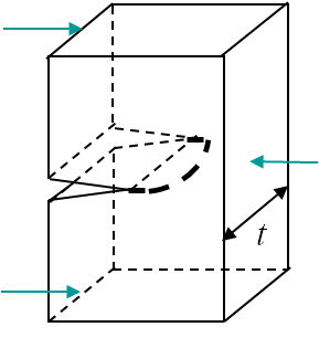
Near the border of a specimen the problem state is plane-stress (P-$\sigma$), while it is plane-strain (P-$\varepsilon$) near the center, where the triaxiality is higher. This means that the SIF is larger at the center as there are more constraints (no possible lateral deformations) (see next lecture). This has two consequences:
- The front propagates first at the center, see Picture V.1.
- The SIF measured at fracture is lower for a thick specimen as the P-$\varepsilon$ state dominates, see Picture V.2.
A crude approximation of the thickness $t$ effect on the measured toughness is
\begin{equation} K_{IC}\left(t\right) \simeq K_{IC}\left(t\rightarrow\infty\right) \sqrt{1+\frac{1.4}{t^2}\left(\frac{K_{IC}\left(t\rightarrow\infty\right) }{\sigma_p^0}\right)^4},\end{equation}
were $\sigma_p^0$ is the initial yield stress.
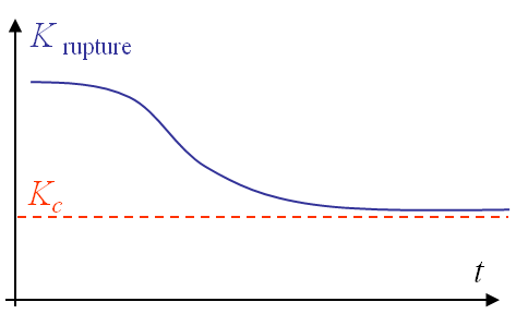
From this observation it appears that the toughness $K_{IC}$ is not dependent on the material only, as the thickness has an effect. To remain conservative, the toughness is defined as the measured value for a "thick-enough" specimen, see Picture V.2.
As a general rule, plane strain and elastic fracture conditions can be assumed if the working zone is small compared to the sample dimensions, including crack length, ligament and thickness. This is the case, as it will be shown in a future lecture, if
\begin{equation} a,\,t > 2.5 \left( \frac{K_c}{\mathbf{\sigma}_p^0} \right)^2.\label{eq:LEFM}\end{equation}
In that case the plane strain state is assumed and the relation (\ref{eq:GCKC}) becomes
\begin{equation} K_{IC} = \sqrt{ \frac{E G_C}{1-\nu^2}}. \end{equation}
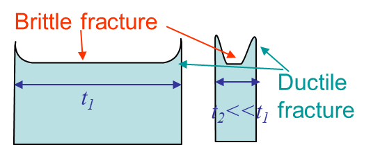
Picture V.3 shows that for thick enough specimen, brittle fracture behavior dominates the crack front. In the following table, one can find the toughness and fracture energy of selected brittle materials (for indication purpose only).
| Material | $K_{IC} \text{[MPa }\cdot\sqrt{\text{m}}\text{]}$ | $G_{C} \text{[J }\cdot\text{m}^2\text{]}$ |
|---|---|---|
| Boroscilicate glass | 0.8 |
9 |
| Alumina 99% polycrystalline | 4 |
39 |
| Zirconia-toughned alumina | 6 |
90 |
| Yttria partially-stabilized zirconia | 13 |
730 |
| Aluminum 7075-T6 | 25 |
7800 |
| AlSiC matric composite | 10 |
400 |
| Epoxy | 0.4 |
200 |
Environmental conditions
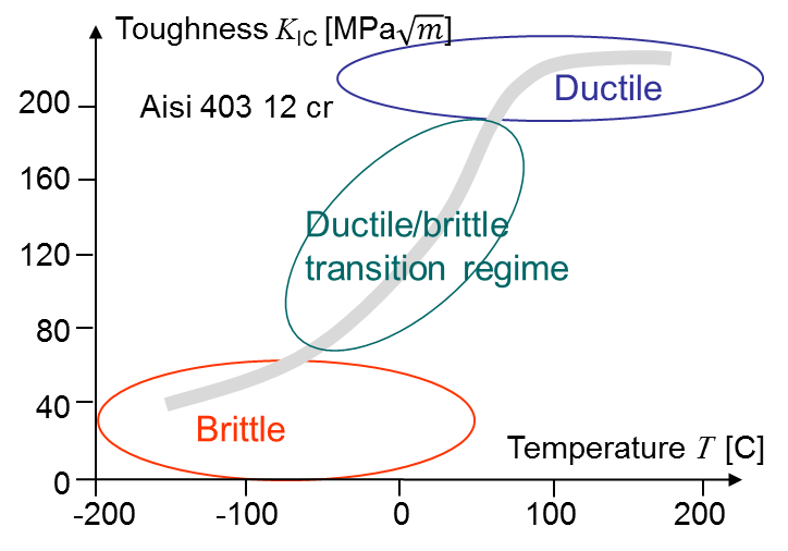
The fracture toughness could aslo depend on the environmental conditions. For example, as discussed before, some materials have a brittle behavior at low temperature and a ductile behavior at high temperature. For such materials the toughness depends on the temperature and there exists a transition region as shown in Picture V.4.
At this stage we are able to determine whether a crack will grow in mode I. But some questions remain: How fast? How far? In which direction? What about other modes? The answers will be part of the next page.
![]()