
Overview > Crack propagation in structures submitted to cyclic loading
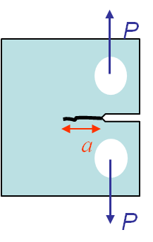
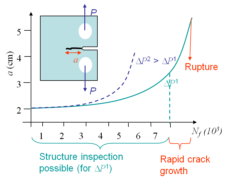
The last concepts of fracture mechanics we need to introduce are related to fatigue. Let us consider a specimen under cyclic loading as described on Picture I.71. The value of $P$ ranges from $P_\text{min}$ to $P_\text{max}$ so that $\Delta P = P_\text{max} - P_\text{min}$. Due to the cyclic loading a crack nucleates at the stress concentration and propagates until failure of the specimen, although at the beginning the SIF remains lower than $K_{IC}$, see Picture I.72. In this overview we will explain the phenomenological explanation of fatigue, and also introduce a way to evaluate the life of a structure with an initial crack subjected to a cyclic loading. We will finish by introducing different design approaches.
Phenomenological explanations
Crack nucleation
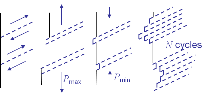
The crack nucleates in a stress concentration area. During the loading of the sample, dislocations move along slip planes until reaching a free surface (or a bulk defect), see Picture I.73, center left. Remember that dislocations are missing atoms, so when they reach the surface this creates a step. During the unloading phase, dislocations can move in the opposite direction but usually it happens on other slip planes, see Picture I.73, center right. After a few cycles one can observe the formation of Persistent Slip Bands (PSBs), see Picture I.73, right. These PSBs are the locations from which the crack can nucleate.
Fatigue crack growth: Stage I.
Once the crack has nucleated, under the cyclic loading condition, it starts to growth along a slip plane of the crystal. The crack thus growths in a direction allowed by the crystallographic orientation.
Fatigue crack growth: Stage II.
During the second stage the crack has passed the first grains layer from the surface. In each grain the crack has to follow their crystallographic orientations. However when the crack size is larger than the size of a few grains, the crack appears as propagating at the macroscopic level in a direction governed by the maximum hoop stress (straight for pure mode I).
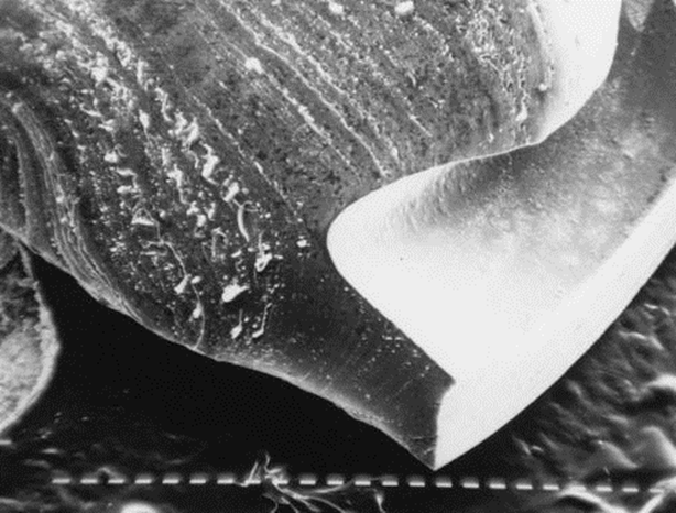
This crack propagation stage is thus a macroscopic propagation stage. It can easily be obseved on fatigue fractured sample under the form of striations (one per cycle) on the failure surface, see Picture I.74.
Fatigue crack growth: Stage III.
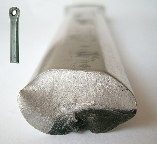
As the crack propagates under the cyclic loading its size increases. While at the beginning of the cyclic loading the SIF remains small compared the material toughness, as $a$ increases the SIF also increases and, at maximum loading $P_{\text{max}}$, becomes close to the toughness $K_{IC}$. At this stage we are back to a classical fracture mechanics problem and the sample will break at once. A fatigue fracture surface thus exhibits two surfaces: striation by fatigue in Stage II and brittle (or ductile) fracture in Stage III, see Picture I.75.
Prediction of the structural life
The question is now how can we predict the evolution of the crack size, and the failure point, in terms of the cycles number. In other words, how can we predict the curves of Picture I.72.
As the crack loading remains small during fatigue problems, the SSY assumption usually holds during some intervals of the crack growth or even until failure, depending on the case. As at the macro-scale the life of the structure with an initial crack size $a$ is observed to depend on the loading $\Delta P$ and on $\frac{P_\text{max}}{P_\text{min}}$ only, the SSY assumption allows us to say that the conditioning parameters are $\Delta K$ and $R = \frac{K_\text{max}}{K_\text{min}}$. Indeed from the SIFs equations we observed a linearity in $\Delta P$ of $\Delta K$. Therefore the evolution of the crack size obeys to
\begin{equation} \frac{d a}{d N_f} = f\left(\Delta K, R\right). \label{eq:dadN}\end{equation}
With the knowledge of this curve it is possible to determine for the number of cycles a structure can sustain before being replaced and to schedule the inspection intervals. Note that the uncertainty on this curve can reach several (tens of) percent, so regular intervals are thus required to validate or modify the prediction.
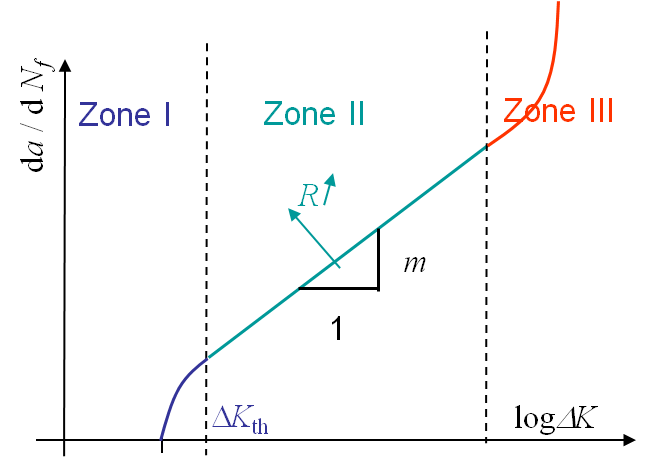
What remains to be defined now is the form of $f\left(\Delta K, R\right)$ in (\ref{eq:dadN}). Experimentally it has been found that this function follows the curve shown in Picture I.76.
Crack propagation in Stage I
Experimentally, it has been observed that if $\Delta K < \Delta K_\text{th}$, where $\Delta K_\text{th}$ the crack growth is in average smaller than one atomic spacing per cycle. Such a crack is considered as dormant. The value of $\Delta K_\text{th}$ is the fatigue threshold and depends on the material but also on the loading ratio $R$.
If $\Delta K > \Delta K_\text{th}$, the crack will propagate until reaching the stage II.
For steel, $\Delta K_\text{th}$ is between 2 and 5 $\text{MPa}\cdot\sqrt{\text{m}}$, but for steel in sea water, $\Delta K_\text{th}$ is between 1 and 1.5 $\text{MPa}\cdot\sqrt{\text{m}}$. This means that the environmental conditions in which the material is considered are very important.
Crack propagation in Stage II
\begin{equation} \frac{d a}{d N_f} = C \Delta K ^m.\label{eq:Paris} \end{equation}
This law is characterized by two parameters $C$ and $m$ which depend on the material and on the loading ratio $R$. For steel, $C \approx 0.1\times 10^{-11}$ $\text{m}\cdot\left(\text{MPa}\cdot\sqrt{\text{m}}\right)^{-m}$ and $m \approx$ 4. For steel in sea water, these values change a lot: $C \approx 1.6 \times 10^{-11}$ $\text{m}\cdot\left(\text{MPa}\cdot\sqrt{\text{m}}\right)^{-m}$ and $m \approx$ 3.3. This means that the environmental conditions in which the material is considered are very important. Note that the units of $C$ are cumbersome as they depend on the coefficient $m$.
When applying the Paris law, it is important to remember that $K$ depends on the crack size. Thus $\Delta K$ should be replaced by its complete expression when integrating to get $a(N_f)$. For instance, for Mode I in an infinite plate, we have:
\begin{equation} K_I = \sigma_\infty \sqrt{\pi a}, \end{equation}
and $\Delta K$ is given by:
\begin{equation} \Delta K = \left(\sigma_{\infty,\text{max}}-\sigma_{\infty,\text{min}}\right) \sqrt{\pi a}. \end{equation}
Crack propagation in Stage III
In this zone the crack grows rapidly until failure of the structure. The failure is reached as soon as the crack size reaches $a_f$ such that $K(P_\text{max},\,a_f)$ is equal to $K_c$.
Design methods
When an engineer has to design a structure submitted to cyclic loading, there exist different design approaches, appeared chronlogically in time with the improvment of fracture mechanics theory:
- Infinite life design. In this case we always ensure that the stress amplitude $\sigma_a$ is lower than the endurance limit $\sigma_e$ so that the life is "infinite". In practice this design is never used as it is economically inefficient.
- Safe life design. For this design we make sure that no cracks appear before a given number of cycles (the structure life) is reached. At the end of the expected life the component is changed even if no failure has occurred. This method clearly puts the emphasis on cracks prevention: a crack free structure is assumed. The number of cycles is determined by the the total life approach. Nowadays this method is used for rotating structures vibrating with the flow as turbine blades. Indeed because of the very high number of cycles to be sustained by these structures, once a crack has formed the remaining life time is very short in hours. However a particular attention should be paid to the quality of the components as the structure is assumed to be defect-free.
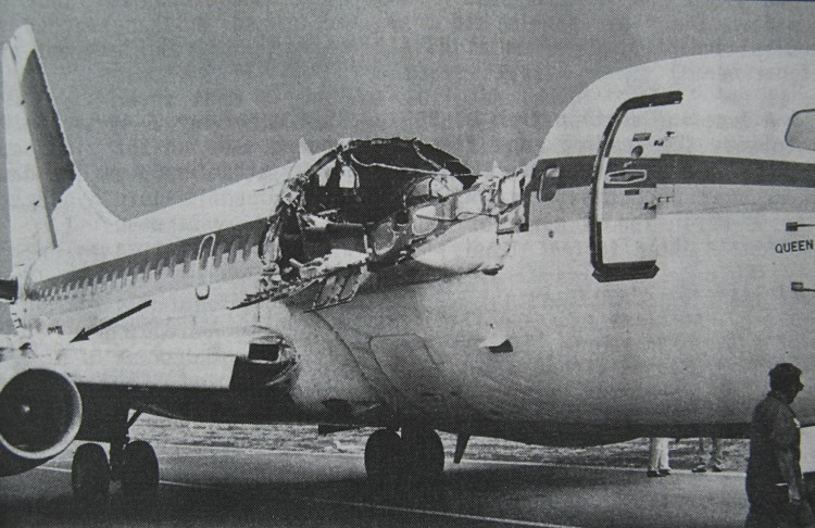
- Fail Safe design. The philosophy of this design is to consider failure of a component as possible. However the design is such that there remains enough integrity to operate the structure safely. This means that in such a design the crack path has to be determined and crack arresters have to be added to the structure. To avoid too many critical cracks at once, it is necessary to regularly check the structure. The difference with the approaches described before is that one focuses more on crack arrest than on crack initiation. An example of such a design is the Boeing 737. In 1988 the Aloha Airlines flight 243 suffered from a production defect: two fuselage plates had not been glued, allowing sea water to induce corrosion, resulting in a loading of the rivets due to the increase of volume between the plates (due to corrosion). This led to fatigue of the rivets, which failed. But due to the design, the crack followed the defined path as can be seen in Picture I.77, and the plane could still be operated.
-
Damage tolerant design This design is more recent and is used for recent aircraft structures. This method assumes that cracks are present from the beginning of service. To be able to predict the life time of the structure it is necessary to be able to characterize the significance of the existing cracks. To do so one needs to determine the initial crack sizes through non-destructive inspections. Once the critical crack sizes are known the Paris-Erdogan law is used to estimate the crack growth rate during service and thus the life of the structure. Conservative inspection intervals, like every so many years or after a certain amount of flight hours, are thus scheduled to validate or correct the predictions. During these inspections one verifies the crack growth, and predicts the end of life af. If this end of life is too close in the future, the part is either replaced or an implemented repair-rehabilitation strategy is planned. Different non-destructive inspections techniques are based on:
- Optics,
- X-Rays,
- Ultrasound ...
This ends the overview of what will be seen during the different lectures. As you could see fracture mechanics uses many new concepts, which at the first glimps seem to be very complex, but will look simpler at the end of the class.