
\(\newcommand{\cauchy}{\boldsymbol{\sigma}}\) \(\newcommand{\strain}{\boldsymbol{\varepsilon}}\) \(\newcommand{\uV}{\boldsymbol}\) \(\newcommand{\uT}{\mathbf}\) \(\newcommand{\defu}{\boldsymbol{u}}\)
$J$-integral > Evaluation of the J-integral
In the previous section, we have discussed the interest of being able to evaluate the $J$-integral for cracked bodies made of elasto-plastic materials. In this section we present different possible approaches.
Numerical methods
Since we have detailed the different approaches in the numerical method part, we refer to that section.
Energetic approaches
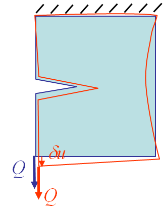
We have previously developed the evaluation of the energy release rate of a cracked body subjected to
- A dead load, see also Picture IX.3;
- A prescribed displacement, see also Picture IX.5;
- A general loading condition.
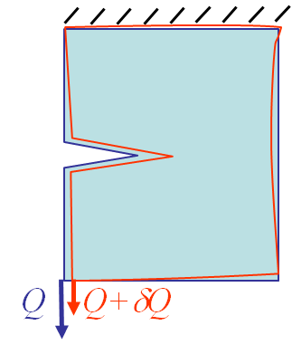
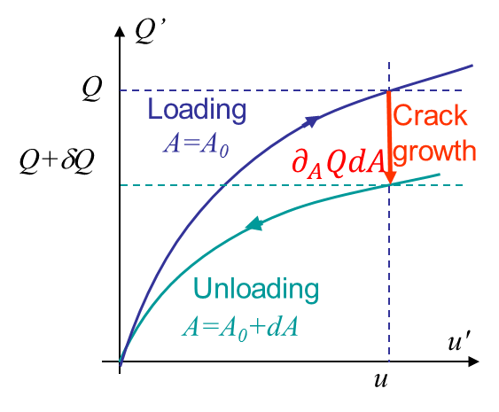
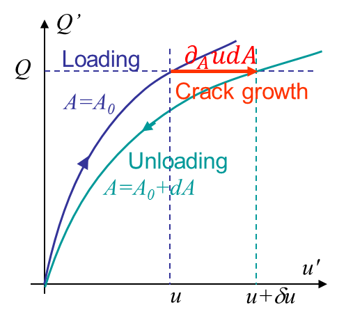
For the two former cases, we have seen that the two same bodies with the same loading condition, but with two different crack surface areas $A$ exhibit the curves in Picture IX.4 for the dead load case and in in Picture IX.6 for the prescribed displacement case. The area in between the blue and green curves corresponds to $G dA$, and thus to $JdA$.
The energetic method consists thus in evaluating the area between two loading curves. Practically the crack growth curve in red and the unloading curve in green are purely virtual, and two samples of two different surface areas $A$ are considered. These two samples can be obtained
- Either experimentally by manufacturing two different samples (this is not a crack propagation test); or
- Numerically by computing the curves $u(a,\,Q)$ using the finite element method e.g.
Experimental methods
Multiple-specimen testing method
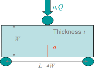
In this approach developed by Begley & Landes in 1972, we consider 4 identical notched samples, such as the single notched specimen illustrated in Picture IX.7, but with four different crack lengths: $a_1<a_2<a_3<a_4$. The four samples are loaded under displacement control $u$, and the force evolution $Q(a,\,u)$ is recorded. There is no crack propagation occurring during the loading: these are not fracture tests.
The methodology allowing the $J$-integral to be evaluated is the following:
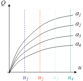
- First the recorded force evolutions $Q(a,\,u)$ are reported as in Picture IX.8, for the 4 cracked specimens of crack length $a_j$, and the loads are measured at four different displacements $u_i$ yielding $Q_i^j=Q(a_j,\,u_i)$;
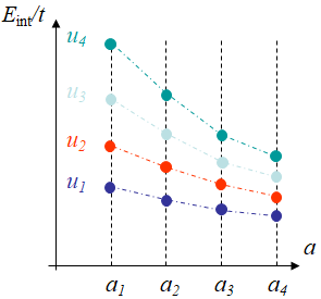
- Since the loading remains proportional an internal potential can be defined, and the internal energy \begin{equation} E_{int_i}^j =\int_0^{u_i}Q(a_j,\,u')du',\end{equation} can be evaluated at four displacement levels $u_i$ and for the 4 samples of crack length $a_j$. These energies per unit thickness $t$ are then reported on Picture IX.9.
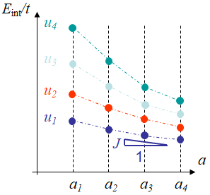
- Since the internal energy evolutions are evaluated at prescribed displacements, using the definition of the energy release rate, the $J$-integral is the slope of the internal energy per unit thickness with respect to the crack length \begin{equation} J=- \frac{1}{t}\frac{\partial E_{int}}{\partial a}|_u\end{equation} as illustrated in Picture IX.10.
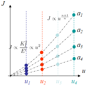
- Finally, the 4$\times$4 evaluated $J$-integrals are reported in terms of the displacement evolution, with values evaluated at the 4 displacements $u_i$, for the 4 crack lengths $a_j$ following Picture IX.11.
This method allows the $J$-integral to be evaluated experimentally, and does not need to actually propagate cracks. However, several specimens need to be tested. We note in Picture IX.11 that at small displacementsthe LEFM solution should be recovered and $J\propto K_I^2$; since $K_I$ is linear with the displacement in linear elasticity, we recover $J\propto u^2$. At larger displacements, elasto-plasticity develops, and the HRR solution should be recovered, in which case one has $J\propto u^{\frac{n+1}{n}}$ with $n$ the hardening modulus.
Deeply notched specimen testing
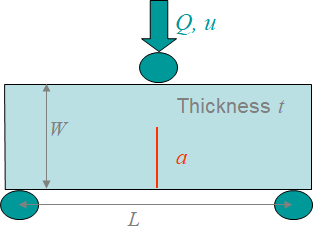
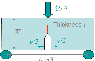
In this study we consider a specimen with an extended notch, see e.g. Picture IX.12. We will see later in this section that for such a notch we can assume that the ligament is fully plastic, allowing some assumptions to be made. Besides, we assume that the specimen is loaded under force control condition.
Without assuming any particular size of the specimen, we can conduct a non-dimensional analysis of the problem.
- The problem is characterized by 9 inputs with the following dimensions:
- The length $L$, with $[L]=\text{m}$;
- The width $W$, with $[W]=\text{m}$;
- The ligament length $L-a$, with $[L-a]=\text{m}$;
- The thickness $t$, with $[t]=\text{m}$;
- The Young's modulus $E$, with $[E]=\text{kg}\cdot\text{m}^{-1}\cdot\text{s}^{-2}$;
- The Yield stress $\sigma_p^0$, with $[\sigma_p^0]=\text{kg}\cdot\text{m}^{-1}\cdot\text{s}^{-2}$;
- The applied load $Q$, with $[Q]=\text{kg}\cdot\text{m}\cdot\text{s}^{-2}$;
- The Poisson ratio $\nu$, with $[\nu]=-$; and
- The hardening exponent $n$, with $[n]=-$.
- Three dimensions are involved in the inputs:
- The distance $\text{m}$;
- The mass $\text{kg}$; and
- The time $\text{s}$.
As a consequence, the Buckingham $\pi$ theorem states that any (non-dimensional) output can be written as a function in terms of 9-3=6 independent nondimensional variables. In the problem depicted in Picture IX.12, the output of interest is the deflection $u$, or in the non-dimensional form $\frac{u}{L}$, that is thus written as
\begin{equation} \frac{u}{L} = f\left(\frac{QL}{Et\left(W-a\right)^2},\,\frac{E}{\sigma_p^0},\, \frac{L}{W-a},\,\frac{W}{W-a},\,n,\,\nu\right), \label{eq:pi1}
\end{equation}
where the 6 non-dimensional variables are chosen as $\frac{QL}{Et\left(W-a\right)^2},\,\frac{E}{\sigma_p^0},\, \frac{L}{W-a},\,\frac{W}{W-a},\,n,$ and $\nu$.
Besides, as recalled in the energetic approach, the energy release rate, and thus the $J$-integral before crack propagation, is the area between the curves of Picture IX.4, i.e.
\begin{equation} J=\frac{1}{t}\int_0^Q \partial_a u\left(Q',\,a\right) dQ' ,\label{eq:Jdeadload}\end{equation}
with $u$ given by Eq. (\ref{eq:pi1}). Derivation of Eq. (\ref{eq:pi1}) with respect to the crack size yields
\begin{equation} \partial_a u = L\left(\frac{2QL}{Et\left(W-a\right)^3}\partial_{\frac{QL}{Et\left(W-a\right)^2}} f + \frac{L}{\left(W-a\right)^2}\partial_{\frac{L}{W-a}} f+\frac{W}{\left(W-a\right)^2}\partial_{\frac{W}{W-a}} f \right),\label{eq:pi2}\end{equation}
where we have used the classical rules of multi-variate function derivatives. However, since only one variable of Eq. (\ref{eq:pi1}) involves the load $Q$, one has
\begin{equation} \partial_Q u = L\left(\frac{L}{Et\left(W-a\right)^2} \partial_{\frac{QL}{Et\left(W-a\right)^2}} f \right),\label{eq:pi3} \end{equation}
or again
\begin{equation} \partial_{\frac{QL}{Et\left(W-a\right)^2}} f=\frac{Et\left(W-a\right)^2}{L^2} \partial_Q u, \label{eq:pi4} \end{equation}
and Eq. (\ref{eq:pi2}) becomes
\begin{equation} \partial_a u =\frac{2Q}{\left(W-a\right)} \partial_Q u + \frac{L^2}{\left(W-a\right)^2}\partial_{\frac{L}{W-a}} f+\frac{LW}{\left(W-a\right)^2} \partial_{\frac{W}{W-a}} f .\label{eq:pi5} \end{equation}
Introducing Eq. (\ref{eq:pi5}) in Eq. (\ref{eq:Jdeadload}) yields a new expression of the $J$-integral:
\begin{equation} J= \frac{1}{t}\int_0^Q \frac{2Q'}{\left(W-a\right)} \partial_{Q'} u dQ'+\frac{1}{t}\int_0^Q \frac{L^2}{2\left(W-a\right)^2}\partial_{\frac{L}{W-a}} f dQ'+\frac{1}{t}\int_0^Q\frac{LW}{2\left(W-a\right)^2}\partial_{\frac{W}{W-a}} f dQ'\,, \label{eq:pi6}\end{equation}
which can be rewritten as
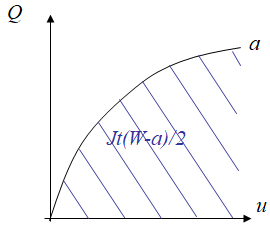
\begin{equation} J= \frac{2}{t\left(W-a\right)}\int_0^{u} Q\left(u'\right) du'+I_1+I_2\label{eq:Jpi}. \end{equation}
Eq. (\ref{eq:Jpi}) involves two integrals $I_1$ and $I_2$ that cannot be written in a closed-form. However, in case they can both be neglected, the expression (\ref{eq:Jpi}) becomes simple since it is proportional to the area below the loading curve as illustrated in Picture IX.13.
The question that now arises, is when can we neglect these two integral terms, and we will see that this is the reason of considering deeply notched specimens.
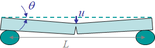
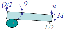
Let us consider the deeply notched bend specimen illustrated in Picture IX.14, in which the ligament of length $W-a$ is fully plastic. If the crack is deep enough, there is a plastic hinge localized between the loading point and the crack tip.
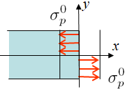
We now assume that the material is perfectly plastic, i.e. the hardening modulus $n\rightarrow \infty$. In that case, a beam under bending exhibits the stress distribution reported in Picture IX.15, in which $\sigma_p^0$ is the yield stress of the material. Indeed, during bending the classical bi-triangular stress profile first develops in the elastic regime, until the yield stress is reached at the beam outer skin. The elastic part then progressively reduces while the elasto-plastic parts are reaching for the beam inertia center. For perfectly plastic materials, since there is no hardening, the stress profiles finally exhibit a bi-rectangular shape, for which the bending moment $M$, see Picture IX.16, that can be balanced is maximum: this is a plastic hinge.
Since the plastic hinge localizes at the ligament of length $L-a$, the maximum bending moment reads
\begin{equation} M = 2 t \int_0^{\frac{W-a}{2}}\sigma y dy = \frac{t \sigma_p^0\left(W-a\right)^2}{4},\label{eq:momentplastichinge} \end{equation}
as seen by Picture IX.15. Moreover, static equilibrium, see Picture IX.16, implies $M=\frac{QL}{4}$, and the last equation, which also reads $M \propto \left(W-a\right)^2$, implies $ Q \propto \left(W-a\right)^2$. As a result we have the following derivative:
\begin{equation} \partial_a Q =-\frac{2}{W-a} Q \label{eq:dQdaDeepNotch}.\end{equation}
As recalled in the energetic approach, the energy release rate, and thus the $J$-integral before crack propagation, is the area between the curves of Picture IX.2, i.e.
\begin{equation} J = -\frac{1}{t}\int_0^u \partial_aQ du' ,\label{eq:Jdeepnotch1}\end{equation}
or using Eq. (\ref{eq:dQdaDeepNotch}),
\begin{equation} J = -\frac{1}{t}\int_0^u \partial_aQ du' = \frac{2}{t\left(W-a\right)}\int_0^u Q\left(u'\right) du'. \label{eq:Jdeepnotch}\end{equation}
Comparing Eq. (\ref{eq:Jdeepnotch}) with Eq. (\ref{eq:Jpi}) shows that for a deeply single edge notched bend specimen made of a perfectly plastic material, the two integral terms $I_1$ and $I_2$ are indeed zero.
For other geometries and materials, this observation is not always true, although for single edge notched bend specimen with $0.4<\frac{a}{W}<0.6$ their contribution of the two integral terms $I_1$ and $I_2$ can generally be neglected as it can be shown by comparison with multiple specimen testing as shown by " Castro P, Spurrier P, and Hancock J (1984) Comparison of J testing techniques and correlation J-COD using structural steel specimens, International Journal of Fracture 17, 83-95". However this situation is far from being general, motivating the development of the $\eta$-factor approach.
$\eta$-factor approach
In the previous section, we have seen that a non-dimensional analysis provides the expression (\ref{eq:Jpi}) of the $J$-integral, which would be easy to be evaluated if there were not the two integral terms $I_1$ and $I_2$. In particular cases, these two terms vanish and one has Eq. (\ref{eq:Jdeepnotch}). The idea behind the $\eta$-factor approach is to substitute the effect of the two integrals by modifying the numerator $2$ by an unknown ratio, with for rigid plastic materials
\begin{equation} J = \frac{\eta_J}{t\left(W-a\right)}\int_0^u Q\left(u'\right) du', \label{eq:etaJrigplast}\end{equation}
where $\eta_J$ depends on the geometry and loading conditions, on the crack ratio $\frac{a}{W}$ and on the material hardening $n$.
However, for an elasto-plastic material, there exists a reversible energy stored in the sample during its loading, see the expression of an internal potential of an elasto-plastic material under proportional loading. The method has thus to be adapted accordingly. Let us consider a cracked sample such as in Picture IX.17 made of an elasto-plastic material subjected to a prescribed load $Q$. During the proportional loading, either the deflection at the loading point $u$ or the crack mouth opening $v$ is recorder. Usually the latter one is measured in a more accurate way and is thus favored. Since the material is elasto-plastic, the elastic part of the deflection and of the opening can be recovered in case of unloading, allowing writing
\begin{equation}u = u_e+u_p \text{ and } u = u_e+u_p,\label{eq:elasticplasticopening}\end{equation}
where the subscript $''e''$ is used for the reversible (elastic) part and the subscript $''p''$ is used for the irreversible (plastic) part.
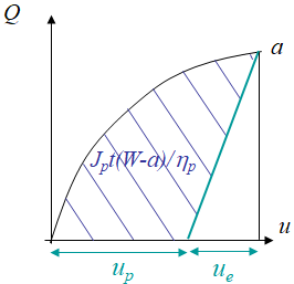
Because of the existence of the elastic part in the deflection, Eq. (\ref{eq:etaJrigplast}) is no longer valid since it refers to the energy dissipated by plasticity only. The correct expression thus reads
\begin{equation} J_p = \frac{\eta_p}{t\left(W-a\right)}\left(\int_0^u Q du'- \frac{Qu_e}{2}\right), \label{eq:etaJplast} \end{equation}
where $J_p$ is the plastic part of the $J$-integral, and which evaluation is illustrated in Picture IX.18. The total $J$-integral is thus obtained by considering the elastic part $J_e$ evaluated using the LEFM assumption, leading to
\begin{equation} J = J_e+J_p = \frac{K_I^2\left(a_\text{eff}\right)}{E'} + \frac{\eta_p}{t\left(W-a\right)}\left(\int_0^u Q du'- \frac{Qu_e}{2}\right),\label{eq:Jeta} \end{equation}
where $\eta_p$ is the unknown coefficient. Finally, as previously said, the measure of the crack mouth opening is more accurate than that of the deflection. A similar expression can thus be obtained in terms of $v$, under the form
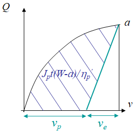
\begin{equation} J = J_e+J_p = \frac{K_I^2\left(a_\text{eff}\right)}{E'} +\frac{\eta_p'}{t\left(W-a\right)}\left(\int_0^v Q dv'- \frac{Qv_e}{2}\right),\label{eq:Jetaprim}\end{equation}
with the graphical interpretation illustrated in Picture IX.19. In this latter expression, $\eta_p'$ is in all generality different from $\eta_p$.
Finally, what remains to be evaluated is the $\eta_p$ (or $\eta_p'$) factor. To this end, a finite element model of the sample is built. Two analyzes are then performed:
- A non-linear finite element analysis in which:
- The elasto-plastic material response is characterized from uni-axial tension tests (performed on uncracked specimens);
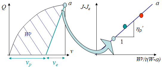
- The specimen is loaded incrementally, and at each increment corresponding to the color bullets of Picture IX.20, the total $J$-integral is numerically evaluated;
- At each load increment, the plastic work is evaluated using \begin{equation} W^p = \int_0^v Q dv'- \frac{Qv_e}{2}.\label{eq:Wp}\end{equation}
- A linear elastic finite element analysis is performed with the same load increments, and at each load increment:
- The elastic $J$-integral $J_e$ is evaluated from the stress intensity factor $K$;
- The plastic $J$-integral $J_p$ is obtained as $J-J_e$.
Finally, the $\eta_p$ (or $\eta_p'$) factor is directly obtained as the slope of $J_p$ with respect to $\frac{W^p}{t(W-a)}$, as illustrated in Picture IX.20.
We will see in the next section that this so-called $\eta$ approach can be used to derive a practical engineering method to evaluate the $J$-integral.
Engineering approach
Following the argumentation of the previous section, the engineering evaluation of the $J$-integral follows a 2-step approach:
- Evaluation of the plastic contribution $J_p$; and
- Evaluation of the elastic contribution $J_e$;
with the total $J$-integral obtained as
\begin{equation} J = J_e+J_p .\label{eq:Jengineering} \end{equation}
The practical evaluation of the two contributions is detailed in engineering handbooks such as "V. Kumar, M.D. German, C.F. Shih (1981) An engineering approach for elastic-plastic fracture analysis, NP-1931, Research Project 1237-1, General Electric Company", and is summarized here below.
Plastic part $J_p$
In the HRR lecture, we have seen that the asymptotic stress field reads
\begin{equation} \cauchy=\sigma_p^0\left(\frac{J E}{r\alpha\left(\sigma_p^0\right)^2I_n}\right)^{\frac{1}{n+1}}\tilde{\cauchy}\left(\theta,\,n\right) \, ,\label{eq:stress_Jint2} \end{equation}
in which the $J$-integral plays the role of an equivalent "plastic strain intensity factor". Let us now consider a fully plastic crack ligament. This equation is rewritten following
- $J_p$ is used instead of $J$ since we assume a fully plastic case;
- The distance $r$ actually scales with to the ligament length $W-a$;
- The stress $\sigma$ scales with the applied load $Q$; and
- Similarly, the yield stress $\sigma_p^0$ scales with a $Q^0$ defined as the limit load that fully plastifies the ligament.
With these considerations, Eq. (\ref{eq:stress_Jint2}) can be rewritten as
\begin{equation} J_p \propto \frac{\alpha\left(\sigma_p^0\right)^2\left(W-a\right)}{E} \left(\frac{Q}{Q^0}\right)^{n+1}. \label{eq:engineeringJp1} \end{equation}
The proportionality factor actually depends on the geometry, loading case, crack size, and hardening law, leading to expressions such as
\begin{equation}
\begin{cases} J_p &= \frac{\alpha\left(\sigma_p^0\right)^2\left(W-a\right)a}{EW} h_1\left(\frac{a}{W},\,n\right) \left(\frac{Q}{Q^0}\right)^{n+1}\,,\text{ or} \\
J_p &= \frac{\alpha\left(\sigma_p^0\right)^2\left(W-a\right)}{E} h_1\left(\frac{a}{W},\,n\right) \left(\frac{Q}{Q^0}\right)^{n+1}\,,\end{cases}\label{eq:engineeringJp} \end{equation}
where $h_1\left(\frac{a}{W},\,n\right)$ and $Q^0$ are obtained by finite element simulations and $h_1$ is tabulated in handbooks. Similar relations are obtained for the plastic deflection at the loading point $u_p$ and the plastic crack mouth opening $v_p$, as well as for the crack tip opening displacement $\delta_t$.
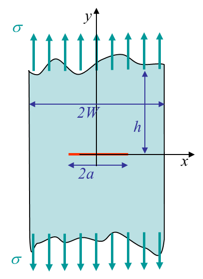
Let us consider the same example as in LEFM: the centered crack in a finite plate illustrated in Picture IX.21. The plastic contributions are written under the form
\begin{equation} \begin{cases} J_p& = \frac{\alpha\left(\sigma_p^0\right)^2\left(W-a\right)}{E} h_1\left(\frac{a}{W},\,n\right) \left(\frac{Q}{Q^0}\right)^{n+1}\,;\\
v_p;\,u_p &= \frac{\alpha\left(\sigma_p^0\right)^2a}{E} h_{2;\,3}\left(\frac{a}{W},\,n\right) \left(\frac{Q}{Q^0}\right)^{n}\,;\\
\delta_t &= \frac{\alpha\left(\sigma_p^0\right)^2\left(W-a\right)a}{EW} h_4\left(\frac{a}{W},\,n\right) \left(\frac{Q}{Q^0}\right)^{n+1}\,.\end{cases} \label{eq:JpCCS} \end{equation}
The limit load reads
\begin{equation}
Q^0 = \begin{cases} 4\left(W-a\right)\frac{\sigma^0_p}{\sqrt{3}} & \text{ in plane-}\varepsilon;\\ 2\left(W-a\right)\sigma^0_p & \text{ in plane-}\sigma, \end{cases} \label{Q0CCS}\end{equation}
and the factor $h_4\left(\frac{a}{W},\,n\right)$ is directly deduced from $h_1\left(\frac{a}{W},\,n\right)$ as $ h_4 = h_1 d_n$ from the crack tip opening displacement $\delta_t$. The other factors are tabulated with some values reported here below for indication purpose only.
| Plane-$\varepsilon$ state | $n=1$ | $n=2$ | $n=3$ | $n=5$ | $n=7$ | |
|---|---|---|---|---|---|---|
| $\frac{a}{W}=\frac{1}{8}$ | $h_1$ | 2.80 |
3.61 |
4.06 |
4.35 |
4.33 |
| $h_2$ | 3.05 |
3.62 |
3.91 |
4.06 |
3.93 |
|
| $h_3$ | 0.303 |
0.574 |
0.840 |
1.300 |
1.630 |
|
| $\frac{a}{W}=\frac{1}{4}$ | $h_1$ | 2.54 |
262 |
2.65 |
2.51 |
2.28 |
| $h_2$ | 2.68 |
2.99 |
3.01 |
2.85 |
2.61 |
|
| $h_3$ | 0.536 |
0.911 |
1.220 |
1.640 |
1.840 |
|
Elastic part $J_e$
The evaluation of the elastic part $J_e$ of the $J$-integral results from the evaluation of the stress intensity factor $K$ following, e.g. the engineering method. However, to account for the process zone, an effective crack size is considered when evaluating the stress intensity factor. One thus has
\begin{equation} J_e = \frac{K_I^2\left(a_\text{eff}\right)}{E'}\,.\label{eq:Jeengineering}\end{equation}
Nevertheless, in order to account for the extended plastic zone that can arise, the evaluation of the effective crack length has to account for the limit load $Q^0$. Therefore, the effective length is still evaluated by the formula
\begin{equation} a_\text{eff}=a+\eta r_p,\label{eq:effcracklengthengineering}\end{equation}
with $\eta$ the ratio of the plastic zone contributing to the effective crack length so that LEFM formula apply and $r_p$ the plastic zone size which is still evaluated as
\begin{equation}\label{eq:rPEngineering} r_p= \left\{ \begin{array}{cc} \frac{n-1}{n+1}\frac{1}{\pi}\left(\frac{K_I\left(a_\text{eff}\right)}{\sigma_p^0}\right)^2 & \text{ in plane-}\sigma ;\\ \frac{n-1}{n+1}\frac{1}{3\pi}\left(\frac{K_I\left(a_\text{eff}\right)}{\sigma_p^0}\right)^2 & \text{ in plane-}\varepsilon\text{.} \end{array}\right. \end{equation}
But, instead of using $\eta=\frac{1}{2}$, the effect of the limit load is accounted for as follows
\begin{equation} \eta = \frac{1}{2\left[1+\left(\frac{Q}{Q^0}\right)^2\right]}.\label{eq:etaEngineering} \end{equation}
![]()