
Numerical Methods > LEFM
Simple Finite Element Simulations
In order to model crack propagation, a simple method is a finite element simulation in which the crack is explicitly modeled with adequate boundary conditions (BCs). The mesh is therefore conforming with the crack lips. Crack propagation can then be evaluated and conducted with the following steps:
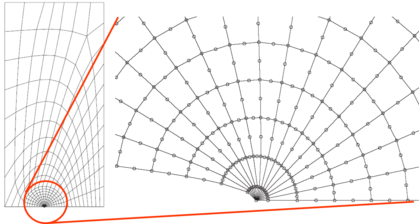
- The structure is meshed in a conforming way with the crack, see Picture VI.1.
- The SIFs ($K_i$) are extracted from the stress or from displacement fields, using the method described in a previous lecture.
- A crack propagation criterion is the applied. For example, the maximal hoop stress criterion $\left( \sqrt{2\pi r} \sigma_{\theta\theta}(r,\theta^*) \right) \geq K_c$ drives the propagation while the direction is obtained with $ \left.\partial_\theta \sigma_{\theta\theta}\right|_{\theta^*} = 0$ & $\left.\partial_\theta^2 \sigma_{\theta\theta}\right|_{\theta^*} = 0$.
- If the crack propagates, the crack tip is moved by $\Delta a$ in the $\theta^*$-direction. A new mesh is therefore required as the crack has changed (since the mesh needs to be conforming).
Despite its simplicity, this method is not used because:
- It involves a large number of remeshing operations (that are time consuming).
- It is not always fully automatic.
- It requires fine meshes and Barsoum elements.
Cohesive elements
Principles
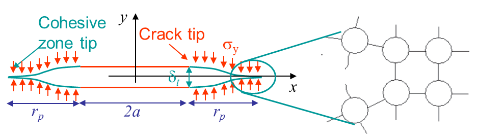
The cohesive method is based on Barenblatt's model, which is an idealization of the brittle fracture mechanisms that involves the breaking of atomic bonding at crack tips (cleavage), see Picture VI.2. As long as they are not separated by a distance $\delta_t$, the crack lips are under attractive forces (see overview lecture).
In the cohesive zone lecture, it will be shown that \begin{equation}J = \int_{0}^{\delta_t} \sigma_y(\delta) d\delta, \end{equation} so the area below the $\sigma - \delta$ curve corresponds to $G_C$ if the crack grows straight ahead.
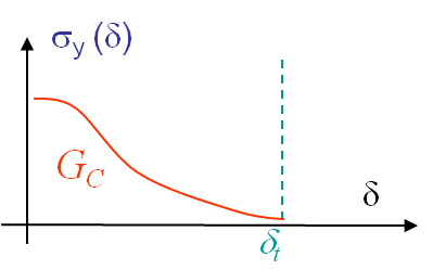
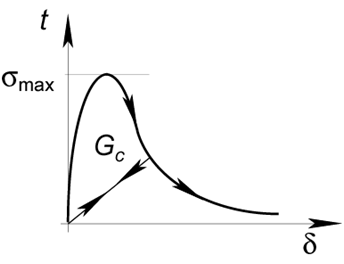
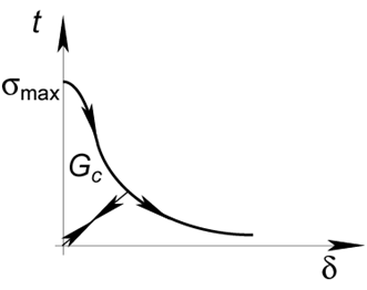
This model is defined trough a cohesive law, see Picture VI.3, which requires only 2 parameters:
- the peak cohesive traction $\sigma_{max}$ (spall strength), and
- the fracture energy $G_C$ , as
the shape of the curves has no effect for brittle materials as long as it is monotonically decreasing.
Computational framework
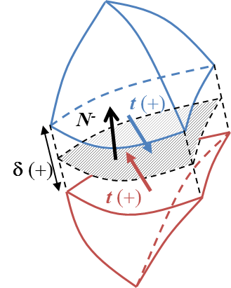
To integrate the cohesive law such as depicted in Picture VI.3, cohesive elements are inserted between two volume elements, see Picture VI.4. In a 3D context, the computation of the opening is calculated with the normal to the interface in the deformed configuration $\mathbf{N^-}$.
The opening, also called jump, between the two volume elements can be decomposed into two parts: the normal opening is equal to $ \delta_n = \max( [\![ \mathbf{u}]\!].\mathbf{N^-},0)$ while the sliding reads $\mathbf{\delta_s} = [\![ \mathbf{u}]\!] - [\![ \mathbf{u}]\!].\mathbf{N^-}\mathbf{N^-}$.
The resulting (or effective) opening is obtained as $ \delta = \sqrt{\delta_n^2 + \beta_c^2 \Vert\delta_s\Vert^2}$ with $\beta_c$ the ratio between the shear and opening critical stress.
A potential $\phi = \phi(\delta)$ can be used to derive the 3D cohesive law, which is also called traction separation law (TSL). The traction (in the deformed configuration) across the crack lips derives from this potential: \begin{equation} \mathbf{t} = \dfrac{\partial \phi}{\partial \mathbf{\delta}} = \dfrac{\partial \phi}{\partial \delta_n} \mathbf{N^-} + \dfrac{\partial \phi}{\partial \delta_s} \dfrac{\partial \mathbf{\delta_s}}{\delta_s}. \end{equation}
Crack insertion
Two approaches can be used to insert the cohesive element, see Picture VI.4, in the finite element mesh.
The first method uses an intrinsic cohesive law:
The pre-failure response and the failure criterion are incorporated within the cohesive law, see Picture VI.5. The cohesive elements can then be inserted since the very beginning of the simulation as they are modeling the pre-failure response. When the maximum traction is reached, the TSL has an irreversible part (during crack opening) and a reversible part (during crack closing).
The main advantage of this method is its ease of implementation: one has only to insert cohesive elements in the initial finite element mesh.
However the method suffers from serious drawbacks:
- The method is not consistent, meaning it does modify the stiffness of the structure which is studied. This is due to the pre-failure stage of the TSL which introduces extra-compliance in the structure.
- As a result, it suffers from mesh dependency [Xu & Needelman, 1994]: the more the number of elements, the more important the artificial compliance of the model.
- The loss of consistency is due to the finite initial slope of the TSL, which modifies the effective elastic modulus of the system and alters the wave propagation.
- Ideally this slope should tend to infinity in order to avoid this problem [Klein et al. 2001], but the method becomes numerically unstable and/or the critical time step is then reduced in explicit time integrations.
This intrinsic method can however be used with an a priori knowledge of the crack path. Indeed, in this case the cohesive elements can be inserted in a limited zone, reducing the artificial compliance issue. For example, the case of delamination in composite laminates can be treated in this way.
The second method uses an extrinsic law:
The extrinsic cohesive law is modeling the failure response of the crack tip only, see Picture VI.6. In this case, the simulation begins with a usual continuous finite element mesh, and when the failure criterion is met ($\sigma \geq \sigma_{max}$) [Ortiz & Pandolfi 1999], interface elements are dynamically inserted in the finite element mesh to integrate the extrinsic TSL.
This method does not suffer from the artifical compliance of the intrinsic method. However, the implementation in 3D is complex especially for parallel simulations, which are mandatory in fracture mechanics.
Improvement: The hybrid Discontinuous Galerkin/Extrinsic Cohesive Law method
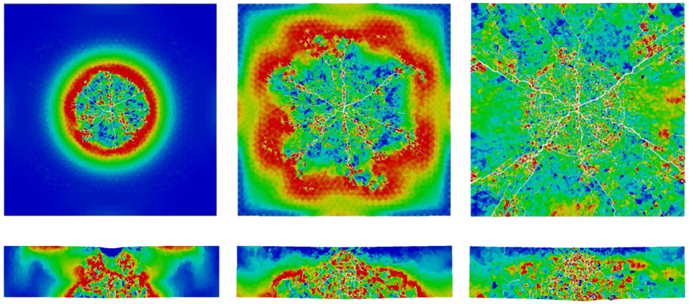
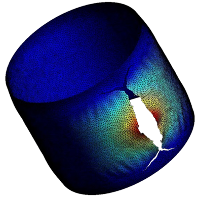
In order to recover the consistency when introducing the interface elements at the beginning of the simulation, the hybrid Discontinuous Galerkin/Extrinsic Cohesive Law method has recently been developed. Examples of simulations can be seen in Pictures VI.7, VI.8, VI.9, and VI.10.
Advantages and drawbacks of the cohesive zone method
Advantages
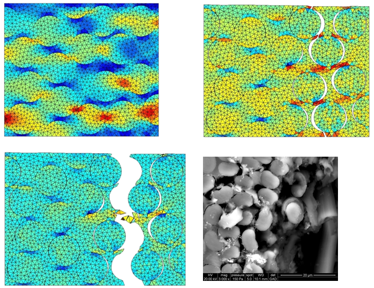
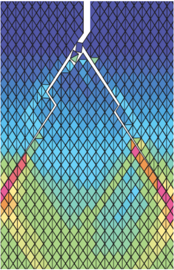
- The method can be mesh independent, see examples of simulations in Pictures VI.7, VI.8, VI.9, and VI.10, if non regular meshes are considered (in the case of regular meshes, preferred crack paths exist, see Picture VI.11).
- It can be used for large problem size with parallel implementations.
- It can automatically account for time scale [Camacho & Ortiz, 1996] (fracture dynamics has not been studied in these classes).
- It is really useful when crack path is already known:
- Debonding of fibers
- Delamination of composite maninates
- ...
- There is no need for an initial crack: the method can detect the initiation of a crack
Drawbacks
- As the crack paths and meshes are conforming, the method requires extra fine meshes to capture the crack path with accuracy.
- As a result, parallelization is mandatory.
- It can be mesh dependent in case of regular meshes as preferred crack paths exist, see Picture VI.11.
The eXtended Finite Element Method
Key principles
The previously presented methods require the finite element mesh to be conforming with the crack. As a results the meshing operation can be complicated and requires fine discretizations. It would thus be advantageous to allow for discontinuities in the finite element model to be non conforming with the mesh as in Picture VI.12.
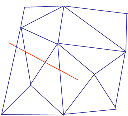
As a reminder, for a classical Finite Element (FE) discretization, the displacement field at coordinates $\xi^i$ is estimated by the sum on the nodes in the set $I$ (11 nodes here in Picture VI.12) of the product of the shape functions with the nodal displacements, i.e.:
\begin{equation} \mathbf{u}_h \left( \xi^i \right) = \sum_{a \in I} N^a \left( \xi^i \right) \mathbf{u}^a, \label{eq:FEinterpolation}\end{equation}
where
- $\mathbf{u}^a$ are the nodal displacements at node $a$,
- $N^a$ are the shape functions associated to the node $a$,
- $\xi^i$ are the reduced coordinates of the finite elements.
However, such interpolation (\ref{eq:FEinterpolation}) of the displacement field cannot account for a discontinuiy. New degrees of freedom are thus required in the model.
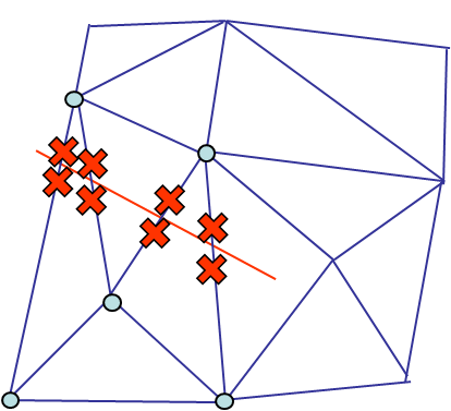
The new degrees of freedom could be introduced by inserting new nodes near the crack tips (red crosses in Picture VI.13), but this would be inefficient as it corresponds to remeshing. Instead, in the eXtended Finite Element Method (XFEM), the new degrees of freedom are introduced through new shape functions in the displacement field interpolation (\ref{eq:FEinterpolation}). As the discontinuity does not affect all the finite elements, only the shape functions related to the nodes linked to the edges that intersect the crack are modified (blue dots in Picture VI.13). The displacement field (\ref{eq:FEinterpolation}) thus becomes:
\begin{equation} \mathbf{u}_h \left( \xi^i \right) = \sum_{a \in I} N^a \left( \xi^i \right) \mathbf{u}^a + \sum_{a \in J} N^a \left( \xi^i \right) F^a \mathbf{u}^{*a},\label{eq:FEModifiedInterpolation} \end{equation}
where
- $J$, a subset of $I$, is the set of nodes whose shape-function support is entirely separated by the crack (5 nodes here, marked with blue dots in Picture VI.13),
- $\mathbf{u}^{*a}$ are the new degrees of freedom related to node $a$,
- $F^a$ are the new shape functions that ought to represent the discontinuity.
The new shape functions $F^a$ have now to be defined so that they can represent the discontinuity in the domain. A logical choice is the Heaviside's function defined such that their evaluation is $+1$ above and $-1$ below the crack. In order to know if we are above or below the crack, the signed-distance from the crack surface should be available for any domain point. This is achieved by defining the level set functions of the domain related to the crack. The displacement field (\ref{eq:FEModifiedInterpolation}) then becomes:
\begin{equation} \mathbf{u}_h \left( \xi^i \right) = \sum_{a \in I} N^a \left( \xi^i \right) \mathbf{u}^a + \sum_{a \in J} N^a \left( \xi^i \right) H(lsn(\xi^i,\xi^{*i})) \mathbf{u}^{*a},\label{eq:FEModifiedInterpolation2} \end{equation}
where
- $H(x)$ is the Heaviside's function, \begin{equation} H(x) = \begin{cases} -1 \text{ if } x \leq 0, \\ +1 \text{ if } x >0, \end{cases} \end{equation}
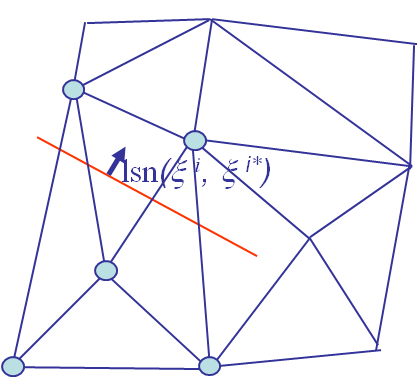
- the normal level set function $lsn(\xi^i, \xi^{i*})$ is defined as the signed distance between a point $\xi^i$ of the domain and its projection $\xi^{i*}$ on the crack surface, see Picture VI.14.
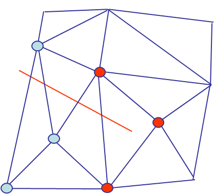
At this point, a discontinuity can be introduced in the mesh and problems with a crack can be solved without the need for a conforming mesh. However, in the context of LEFM one can take advantage of the knowledge of the asymptotic solution expression to improve the accuracy in more efficient way than with a mesh refinement. Toward this end, a new enrichment is needed on the nodes of the elements embedding the crack tip (red dots in Picture VI.15). Indeed, as the asymptotic LEFM solution vanish far away from the crack tip, only closest nodes to the crack tip have to be enriched. The displacement field (\ref{eq:FEModifiedInterpolation2}) thus becomes:
\begin{equation}\begin{cases} \mathbf{u}_h \left( \xi^i \right) &=& \sum_{a \in I} N^a \left( \xi^i \right) \mathbf{u}^a + \sum_{a \in J} N^a \left( \xi^i \right) H(lsn(\xi^i,\xi^{*i})) \mathbf{u}^{*a} \\ &&+\sum_{a \in K} N^a \left( \xi^i \right) \sum_{b} \Psi_b(\xi^i) \mathbf{\psi}_b^a,\end{cases}\label{eq:FEModifiedInterpolation3} \end{equation}
- $K$ a subset of $J$, is the set of nodes of the elements embedding the crack-tip (3 nodes here, marked with red dots in Picture VI.15),
- $\psi_b^a$ is the new $b^{\text{th}}$ degree of freedom number at node $a$,
- $\Psi_b$ is the new $b^{\text{th}}$ shape function.
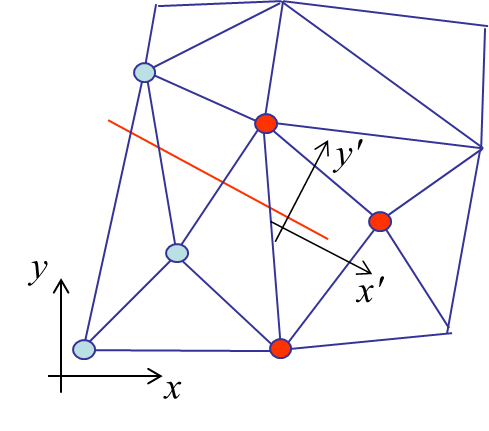
What remain to be defined are the new shape functions $\Psi_b$. Toward this end, the asymptotic displacement field is expressed, in the referential $x'$, $y'$, $z'$ linked to the crack tip, see Picture VI.16, in terms of the three stress intensity factors:
\begin{equation} \begin{cases} \mathbf{u}_{x'} & = \frac{1+\nu}{E} \sqrt{\frac{r}{2\pi}} &\left\lbrace K_I \cos{\frac{ \theta}{2}} \left[\kappa-1+2 \sin^2{\frac{\theta}{2}}\right] +\right.\\ &&\left.K_{II} \sin{\frac{ \theta}{2}} \left[\kappa+1+2 \cos^2{\frac{\theta}{2}}\right] \right\rbrace, \\ \mathbf{u}_{y'} & = \frac{1+\nu}{E} \sqrt{\frac{r}{2\pi}} &\left\lbrace K_I \sin{\frac{ \theta}{2}} \left[\kappa+1-2 \cos^2{\frac{\theta}{2}}\right] + \right.\\ &&\left. K_{II} \cos{\frac{ \theta}{2}} \left[1-\kappa+2 \sin^2{\frac{\theta}{2}}\right] \right\rbrace, \\ \mathbf{u}_{z'} & = \frac{1+\nu}{E} \sqrt{\frac{r}{2\pi}} 2& K_{III} \sin{\frac{\theta}{2}}. \end{cases} \end{equation}
Basic trigonometric relations allow these fields to be rewritten
\begin{equation} \begin{cases} \mathbf{u}_{x'} &=& \frac{1+\nu}{E} \sqrt{\frac{r}{2\pi}} \left\lbrace K_I \cos{\frac{\theta}{2}} \left[ \kappa-1 \right] + K_I \sin{\frac{\theta}{2}} \sin{\theta} + K_{II} \sin{\frac{\theta}{2}} \left[ \kappa+1 \right] + K_{II} \cos{\frac{\theta}{2}} \sin{\theta} \right\rbrace,\\ \mathbf{u}_{y'} &=& \frac{1+\nu}{E} \sqrt{\frac{r}{2\pi}} \left\lbrace K_I \sin{\frac{\theta}{2}} \left[\kappa+1\right] - K_I \cos{\frac{\theta}{2}} \sin{\theta} + K_{II} \cos{\frac{\theta}{2}} \left[1-\kappa\right] + K_{II} \sin{\frac{\theta}{2}} \sin{\theta} \right\rbrace, \\ \mathbf{u}_{z'} & = & \frac{1+\nu}{E} \sqrt{\frac{r}{2\pi}} 2 K_{III} \sin{\frac{\theta}{2}}.\end{cases}\label{eq:manipulation1}\end{equation}
We have then defined four shape functions $\Psi_b$. In the global axes, the shape functions $\Psi_b$ remain the same as $\theta$ is linked to the crack tip direction and we can write
\begin{equation}\begin{cases} \mathbf{u}_x &=& \psi_x^1 \underbrace{ \sqrt{r} \sin{\frac{\theta}{2}} }_{\Psi_1} + \psi_x^2 \underbrace{ \sqrt{r} \cos{\frac{\theta}{2}} }_{\Psi_2} + \psi_x^3 \underbrace{ \sqrt{r} \sin{\frac{\theta}{2}} \sin{\theta}}_{\Psi_3} + \psi_x^4 \underbrace{ \sqrt{r} \cos{\frac{\theta}{2}} \sin{\theta} }_{\Psi_4},\\ \mathbf{u}_y &=& \psi_y ^1 \underbrace{ \sqrt{r} \sin{\frac{\theta}{2}} }_{\Psi_1} + \psi_y^2 \underbrace{ \sqrt{r} \cos{\frac{\theta}{2}} }_{\Psi_2} + \psi_y^3 \underbrace{ \sqrt{r} \sin{\frac{\theta}{2}} \sin{\theta}}_{\Psi_3} + \psi_y^4 \underbrace{ \sqrt{r} \cos{\frac{\theta}{2}} \sin{\theta} }_{\Psi_4}\,,\\ \mathbf{u}_z &=& \psi_z ^1 \underbrace{ \sqrt{r} \sin{\frac{\theta}{2}} }_{\Psi_1} + \psi_z^2 \underbrace{ \sqrt{r} \cos{\frac{\theta}{2}} }_{\Psi_2} + \psi_z^3 \underbrace{ \sqrt{r} \sin{\frac{\theta}{2}} \sin{\theta}}_{\Psi_3} + \psi_z^4 \underbrace{ \sqrt{r} \cos{\frac{\theta}{2}} \sin{\theta} }_{\Psi_4}. \end{cases}\label{eq:manipulation2} \end{equation}We have thus 12 new degrees of freedom $\psi_b^a$ on the LEFM-enriched nodes. Note that as $\Psi_1$ is discontinuous, the Heaviside functions are not required anymore on the nodes in the subset $K$. The enriched displacement field (\ref{eq:FEModifiedInterpolation3}) finally becomes
\begin{equation} \begin{cases}\mathbf{u}_h \left( \xi^i \right) &=& \sum_{a \in I} N^a \left( \xi^i \right) \mathbf{u}^a + \sum_{a \in J} N^a \left( \xi^i \right) H(lsn(\xi^i,\xi^{*i})) \mathbf{u}^{*a} +\\ && \sum_{a \in K} N^a \left( \xi^i \right) \sum_{b=1}^4 \Psi_b\left(r(\xi^i), \theta(\xi^i)\right) \mathbf{\psi}_b^a.\end{cases}\label{eq:xFEMInterpolation} \end{equation}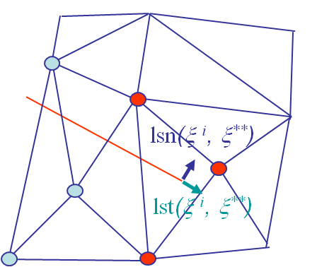
In order to evaluate the new shape functions $\Psi_b\left(r(\xi^i), \theta(\xi^i) \right)$, both the distance $r$ from the crack tip and the direction $\theta$ from the crack tip tangent have to be evaluated, see Picture VI.17. Toward this end, the normal and tangential signed distances from the crack tip have to be obtained through the level set functions. The values of $r$ and $\theta$ are then evaluated by:
\begin{equation} \begin{cases} r &=& \sqrt{lsn(\xi^i,xi^{**})^2 + lst(\xi^i,xi^{**})^2}, \\ \theta &=& \pm \arctan{ \frac{lsn(\xi^i,x^{**})} {lst(\xi^i,x^{**})}}, \end{cases} \end{equation}
where
- the normal level set function $lsn(\xi^i, \xi^{i**})$ is defined as the normal signed distance between a point $\xi^i$ of the domain and the crack tip, see Picture VI.17,
- the tangent level set $lst(\xi^i,xi^{**})$ is defined as the tangential signed distance between a point $\xi^i$ of the domain and the crack tip $\xi^{**}$, see Picture VI.17.
With this framework, the displacement and stress fields of a domain embedding a crack can be computed using non-conforming mesh discretizations. The next step is now to evaluate whether the crack will propagate or not, and if so in which direction.
SIFs computation
In the LEFM context, the crack propagation can be assessed from the computation of the SIFs. Toward this end, the SIFs could be deduced from the new degrees of freedom $\psi_b^a$. Indeed, comparing the displacement fields (\ref{eq:manipulation1}), e.g. in the $x'$-direction linked to the crack tip,
\begin{equation} \mathbf{u}_{x'} = \frac{1+\nu}{E} \sqrt{\frac{r}{2\pi}} \left\lbrace K_I \cos{\frac{\theta}{2}} \left[ \kappa-1 \right] + K_I \sin{\frac{\theta}{2}} \sin{\theta} + K_{II} \sin{\frac{\theta}{2}} \left[ \kappa+1 \right] + K_{II} \cos{\frac{\theta}{2}} \sin{\theta} \right\rbrace, \end{equation}
with the formulation (\ref{eq:manipulation2}), e.g. in the $x'$-direction linked to the crack tip
\begin{equation} \mathbf{u}_{x'} = \psi_{x'}^1 \underbrace{ \sqrt{r} \sin{\frac{\theta}{2}} }_{\Psi_1} + \psi_{x'}^2 \underbrace{ \sqrt{r} \cos{\frac{\theta}{2}} }_{\Psi_2} + \psi_{x'}^3 \underbrace{ \sqrt{r} \sin{\frac{\theta}{2}} \sin{\theta}}_{\Psi_3} + \psi_{x'}^4 \underbrace{ \sqrt{r} \cos{\frac{\theta}{2}} \sin{\theta} }_{\Psi_4}, \end{equation}
shows the relationship between the degrees of freedom $\psi_{b'}^a$ expressed in the referential linked to the crack tip and the SIFs $K_i$:
\begin{equation} \begin{cases} K_I&=&\frac{\psi_{x'}^3\sqrt{2\pi}E}{1+\nu},\\K_{II}&=&\frac{\psi_{x'}^4\sqrt{2\pi}E}{1+\nu},\\K_{III}&=&\frac{\psi_{z'}^1\sqrt{2\pi}E}{1+\nu}.\end{cases}\end{equation}
However, this way of proceeding is not accurate as it is obtained from the displacement field interpolation, whose accuracy strongly depends on the mesh discretization. Therefore the SIFs are usually deduced from the $J$-integral. Toward this end, we apply the methodology described previously, which is summarized by
- The $J$-integral is computed from the finite element resolution;
- Three $J$-integrals are computed for
- the solution displacement field $\mathbf{u}_h$,
- an adequate auxiliary field $\mathbf{u}^{aux}_h$ such that $K^{aux}_i$ is non zero for only $i=1\,,2\,,\,$ or $3$, and
- the combination $\mathbf{u}_h+\mathbf{u}^{aux}$ ,
- The interaction integral is then obtained from $ I^s = J^s - J - J^{aux}$;
- As \begin{equation} I^s = J^s - J - J^{aux}= \frac{2}{E'} \left(K_I K_I^{aux} + K_{II} K_{II}^{aux} \right) + \frac{1}{\mu}K_{III}K_{III}^{aux}, \end{equation} and as $\mathbf{u}^{aux}_h$ was adequately chosen such that only a single $K_{i}^{aux} \neq 0$, the SIF $K_i$ is obtained directly from $I^s$.
Crack propagation criterion
With the developed tools, the xFEM method is an efficient tool to simulate crack propagation. This is achieved as follows
- The structure is meshed first without considering the crack;
- The crack is introduced in the domain through the definition of the level set functions;
- The xFEM is then solved using the enriched displacement field;
- The SIFs ($K_i$) are extracted from the xFEM resolution;
- A crack propagation criterion is the applied; for example, the maximal hoop stress criterion $\left( \sqrt{2\pi r} \sigma_{\theta\theta}(r,\theta^*) \right) \geq K_c$ drives the propagation while the direction is obtained with $ \left.\partial_\theta \sigma_{\theta\theta}\right|_{\theta^*} = 0$ & $\left.\partial_\theta^2 \sigma_{\theta\theta}\right|_{\theta^*} = 0$;
- If the crack propagates, the crack tip is moved by $\Delta a$ in the $\theta^*$-direction; however this does not require a modification of the mesh, but simply a new evaluation of the level set functions;
- When studying fatigue, the crack propagation criterion is replaced by an evaluation of the number of cycles required to move the crack tip by $\Delta a$, for example using $\Delta K$ and the Paris law.
Numerical examples
Resection of a brain tumor [L. Vigneron et al.]
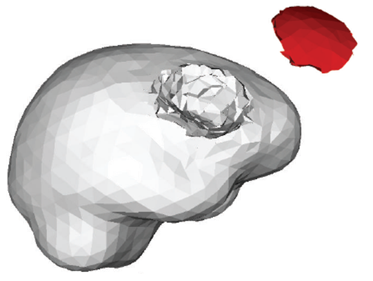
As current neuronavigation systems cannot adapt to changing intraoperative conditions over time an experimental end-to-end system capable of updating 3D preoperative images in the presence of brain shift and successive resections was developed using the XFEM technology. The biomechanical model is deformed using the xFEM in order to model tumor resection without recourse to a conforming mesh, see Picture VI.18.
Advantages and drawbacks
Advantages
- There is no need for a conforming mesh (but the mesh has still to be fine enough near the crack tip in order to describe accurately the crack propagation);
- The simulation is mesh independent;
- The method is computationally efficient.
Drawbacks
- It requires complex radical changes to the hosting FE code:
- New degrees of freedom are added during the simulation ;
- The Gauss-points integration scheme has to be adapted to account for the elements divided by the Heaviside functions (enough integration points on each side of the crack);
- Dirichlet boundary conditions require Lagrange multipliers to be enforced as the nodal displacement on the boundary is now a combinations of the degree of freedom $\mathbf{u}^a$, $\mathbf{u}^{*a}$, and $\psi_b^a$ (for a usual FEM, the nodal displacement is $\mathbf{u}^a$).
![]()