
Crack Growth > Mixed-mode fracture
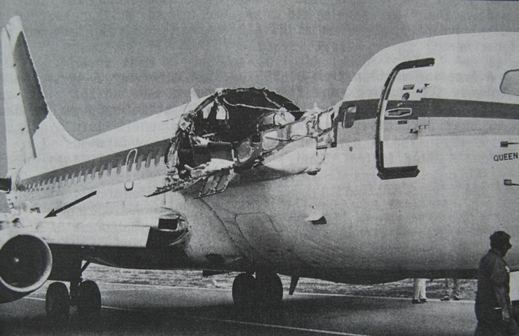
From the previous section, an important question has still to be answered: in which direction does the crack grow? One has to consider the cases of anisotropic and isotropic materials, of mixed-mode loading and of composites. Cracks do follow the path offering the least resistance to propagate. It is therefore convenient to predict this path during the design process -a process called "safe life design", put in practice since the 70's and as illustrated by Aloha Air Boeing 737 incident illustrated in Picture V.11. In 1988 the Aloha Airlines flight 243 suffered from a production defect: two fuselage plates had not been glued, allowing sea water to induce corrosion, resulting in a loading of the rivets due to the increase of volume between the plates (due to corrosion). This led to fatigue of the rivets, which failed. But due to the design, the crack followed the defined path and the plane could still be operated.
In this lecture, we assume an isotropic homogeneous material under mixed-mode loading.
Combination of modes I and II loadings
We have determined whether a crack grows when loaded in mode I. In that case, by symmetry the crack propagates straight ahead. What happens when the loading mode is mixed (for example a combination of mode I and mode II)?
- What is the condition for the crack to grow?
- In which direction would it grow?
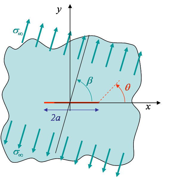
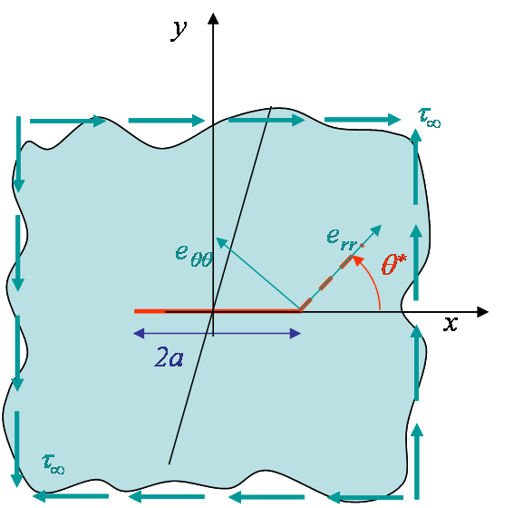
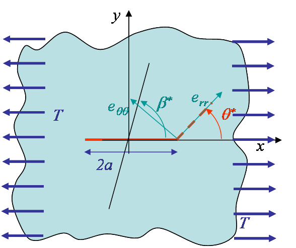
To answer to these questions let us consider the mixed mode loading of Picture V.12, in which the loading direction is oriented with an angle $\beta$ with respect to the crack ($\beta=\frac{\pi}{2}$ corresponding to a pure mode I loading). Under this mixed loading condition the crack propagates with a kink angle $\theta$, and $\theta = 0$ only if it corresponds to a weak plane of the material (bond line in composites e.g.). For an isotropic material this is not the case.
Let us first evaluate the SIFs for such a loading condition:
-
The stress tensor is known in the loading direction and can be expressed in the crack referential using a rotation operation:
\begin{equation} \left(\begin{array}{cc} \mathbf{\sigma}_{xx} & \mathbf{\sigma}_{xy}\\ \mathbf{\sigma}_{xy} & \mathbf{\sigma}_{yy} \end{array}\right)=\left(\begin{array}{cc} \cos{\beta} & \sin{\beta}\\ -\sin{\beta} & \cos{\beta} \end{array}\right)^T \left(\begin{array}{cc} \sigma_\infty & 0\\ 0 & 0 \end{array}\right) \left(\begin{array}{cc} \cos{\beta} & \sin{\beta}\\ -\sin{\beta} & \cos{\beta} \end{array}\right), \label{eq:rotation}\end{equation}
or again:
\begin{equation}\begin{cases} \mathbf{\sigma}_{yy}=\sigma_\infty\sin^2\beta\\ \mathbf{\sigma}_{xy}=\sigma_\infty\sin\beta\cos\beta\\ \mathbf{\sigma}_{xx}=\sigma_\infty\cos^2\beta\end{cases}.\label{eq:sigMixed} \end{equation} -
Assuming an infinite plate, the SIFS corresponding to the modes I and II are respectively obtained from the "yy" and "xy"-stress fields:
\begin{equation}\begin{cases} K_I = \sigma_\infty \sin^2\beta \sqrt{a \pi} \\ K_{II} = \sigma_\infty \sin\beta\cos\beta \sqrt{a \pi}\end{cases}.\label{eq:SIFsMixed} \end{equation}.
To determine the kink angle, we have to come with an assumption. There exist two main methods for determining this angle.
Method of maximum circumferential stress
This method was proposed by Erdogan and Sih (1963) and is based on the assumptions that:
- The crack grows in the direction for which the SIF related to mode I in the new frame is maximal;
- It grows only if this SIF is larger than the toughness measured for a pure mode I loading.
Criterion
As the mode I in the new frame is characterized by the new $\mathbf{\sigma}_{yy}$ in this frame, i.e. $\mathbf{\sigma}_{\theta\theta}$, the crack propagation criterion then reads
\begin{equation} \left(\sqrt{2\pi r}\mathbf{\sigma}_{\theta\theta}\left(r,\,\theta_\star\right)\right) \geq K_{IC} ,\label{eq:MixedPropagation1}\end{equation}
and the direction of propagation $\theta^*$ results from the following system
\begin{equation} \begin{cases}\left.\partial_\theta \mathbf{\sigma}_{\theta\theta}\right|_{\theta^\star} = 0 \\ \left.\partial^2_{\theta\theta} \mathbf{\sigma}_{\theta\theta}\right|_{\theta^\star} < 0 \end{cases},\label{eq:MixedKink1}\end{equation}
The hoop stress
We have now to express the circumferential stress, also called hoop stress, from the asymptotic solution.
- For the 2D mode I loading, the asymptotic solution stress field was found to be
\begin{equation}\begin{cases} \mathbf{\sigma}_{xx} & = & \frac{K_I}{\sqrt{2\pi r}} \cos{\frac{\theta}{2}}\left[1-\sin{\frac{\theta}{2}}\sin{\frac{3\theta}{2}}\right]+\mathcal{O}\left(r^0\right) \\ \mathbf{\sigma}_{yy} &= & \frac{K_I}{\sqrt{2\pi r}} \cos{\frac{\theta}{2}}\left[1+\sin{\frac{\theta}{2}}\sin{\frac{3\theta}{2}}\right]+\mathcal{O}\left(r^0\right)\\ \mathbf{\sigma}_{xy} & = & \frac{K_I}{\sqrt{2\pi r}} \cos{\frac{\theta}{2}}\sin{\frac{\theta}{2}}\cos{\frac{3\theta}{2}}+\mathcal{O}\left(r^0\right)\end{cases},\label{eq:asympModeI} \end{equation} -
For the 2D mode II loading, the asymptotic stress field was found to be
\begin{equation}\begin{cases} \mathbf{\sigma}_{xx} = & - \frac{K_{II}}{\sqrt{2\pi r}} \sin{\frac{\theta}{2}} \left[2 +\cos{\frac{\theta}{2}}\cos{\frac{3\theta}{2}}\right] +\mathcal{O}\left(r^0\right)\\ \mathbf{\sigma}_{yy} = & \frac{K_{II}}{\sqrt{2\pi r}} \sin{\frac{\theta}{2}} \cos{\frac{\theta}{2}}\cos{\frac{3\theta}{2}}+\mathcal{O}\left(r^0\right) \\ \mathbf{\sigma}_{xy} = &\frac{K_{II}}{\sqrt{2\pi r}} \cos{\frac{\theta}{2}}\left[1-\sin{\frac{\theta}{2}}\sin{\frac{3\theta}{2}}\right]+\mathcal{O}\left(r^0\right)\end{cases} \label{eq:asympModeII} . \end{equation} -
Using the superposition principle, as we are in linear elasticity, and omitting the higher order terms, the stress field for the mixed mode loading reads near the crack tip
\begin{equation}\begin{cases} \mathbf{\sigma}_{xx} & = \frac{1}{\sqrt{2\pi r}} \left[K_I\cos{\frac{\theta}{2}}-\frac{K_I}{2}\sin{\theta}\sin{\frac{3\theta}{2}}-2K_{II}\sin{\frac{\theta}{2}}-\frac{K_{II}}{2}\sin{\theta}\cos{\frac{3\theta}{2}} \right] \\ \mathbf{\sigma}_{yy} & = \frac{1}{\sqrt{2\pi r}} \left[K_I\cos{\frac{\theta}{2}}+\frac{K_I}{2}\sin{\theta}\sin{\frac{3\theta}{2}}+\frac{K_{II}}{2}\sin{\theta}\cos{\frac{3\theta}{2}} \right] \\ \mathbf{\sigma}_{xy} & = \frac{1}{\sqrt{2\pi r}} \left[\frac{K_I}{2}\sin{\theta}\cos{\frac{3\theta}{2}}+K_{II}\cos{\frac{\theta}{2}}-\frac{K_{II}}{2}\sin{\theta}\sin{\frac{3\theta}{2}} \right] \end{cases}.\label{eq:asymptMixed}\end{equation} -
Applying a rotation as in (\ref{eq:rotation}) to express the stress tensor in polar coordinates allows the hoop stress $\mathbf{\sigma}_{\theta\theta}$ to be evaluated as
\begin{equation} \mathbf{\sigma}_{\theta\theta}\left(\theta=\beta\right) = \mathbf{\sigma}_{yy} \cos^2{\beta} + \mathbf{\sigma}_{xx} \sin^2{\beta} - 2 \mathbf{\sigma}_{xy} \sin{\beta}\cos{\beta} .\end{equation} -
Using the stress field (\ref{eq:asymptMixed}) in this last equation leads to the expression
\begin{align}\mathbf{\sigma}_{\theta\theta} = & \frac{K_I}{2\sqrt{2\pi r}}\left[2\cos{\frac{\theta}{2}}+\sin{\theta}\cos{2\theta}\sin{\frac{3\theta}{2}}-\sin{2\theta}\sin{\theta}\cos{\frac{3\theta}{2}}\right]+\nonumber \\ & \frac{K_{II}}{2\sqrt{2\pi
r}}\left[\sin{\theta}\cos{2\theta}\cos{\frac{3\theta}{2}}-4\sin^2{\theta}\sin{\frac{\theta}{2}}-2\sin{2\theta}\cos{\frac{\theta}{2}}+\sin{2\theta}\sin{\theta}\sin{\frac{3\theta}{2}}\right] .\end{align}
Using trigonometric identities, this last relation successively reads
\begin{eqnarray} \mathbf{\sigma}_{\theta\theta} &= & \frac{K_I}{2\sqrt{2\pi r}}\left[2\cos{\frac{\theta}{2}}- \sin{\theta}\sin{\frac{\theta}{2}}\right]+\nonumber \\ & &\frac{K_{II}}{2\sqrt{2\pi r}}\left[\sin{\theta}\cos{\frac{\theta}{2}}-4\sin^2{\theta}\sin{\frac{\theta}{2}}-2\sin{2\theta}\cos{\frac{\theta}{2}}\right] \nonumber\\&=&\frac{K_I}{2\sqrt{2\pi r}}\cos{\frac{\theta}{2}}\left[2-\sin^2{\frac{\theta}{2}}\right]+\frac{K_{II}}{2\sqrt{2\pi r}}\left[\sin{\theta}\cos{\frac{\theta}{2}}- 4 \sin{\theta}\cos{\frac{\theta}{2}}\right]. \end{eqnarray} -
The final expression of the hoop stress finally becomes
\begin{equation}\mathbf{\sigma}_{\theta\theta} =\frac{K_I}{\sqrt{2\pi r}}\cos^3{\frac{\theta}{2}}-\frac{3K_{II}}{2\sqrt{2\pi r}}\sin{\theta}\cos{\frac{\theta}{2}}.\label{eq:hoop1} \end{equation} -
Now we can introduce the mixed loading ratio so that
\begin{equation} \cot\beta^\star = \frac{K_{II}}{K_I}. \label{eq:beta}\end{equation}
In the case of the infinite plate problem as in Picture V.12 , $\beta^\star$ corresponds to the loading direction $\beta$ as it can be directly obtained from (\ref{eq:SIFsMixed}). For other cases, it characterizes the ratio between the two loading modes in a general way. The hoop stress (\ref{eq:hoop1}) thus reads
\begin{equation} \mathbf{\sigma}_{\theta\theta} = \frac{K_I}{\sqrt{2\pi r}}\left[\cos^3{\frac{\theta}{2}}- \frac{3\cot{\beta^\star}}{2}\sin{\theta}\cos{\frac{\theta}{2}}\right].\label{eq:hoop} \end{equation}
The kink angle
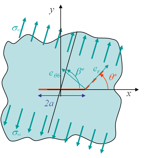
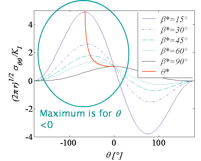
Considering the mixed mode loading characterized by the ratio $\beta^\star$ (\ref{eq:beta}) and illustrated for an infinite plate in Picture V.13, we have established the expression of the asymptotic hoop stress (\ref{eq:hoop}). This field has also a singularity, but the equivalent SIF can be extracted from (\ref{eq:MixedPropagation1}) and its normalized value is reported in Picture V.14 in terms of the polar angle $\theta$ for different values of $\beta^\star$. We can now analyze this result to determine the kink angle $\theta^\star$ which gives the direction of the subsequent crack direction.
- For $\beta^\star = 90$°, the hoop stress is maximum for $\theta=0$ and the crack will thus propagate straight ahead ($\theta^\star = 0$). This case corresponds to a pure mode I loading.
- For $\beta^\star > 0$, the maximum hoop stress is reached for $\theta^\star < 0$, meaning that the crack propagates in a direction closer from the perpendicular with the loading, see Picture V.13.
-
The king angle can be obtained by solving the system (\ref{eq:MixedKink1}) and (\ref{eq:hoop}) which is rewritten
\begin{eqnarray} 0=\left. \partial_\theta\mathbf{\sigma}_{\theta\theta}\right|_{\theta^\star}&=& \frac{K_I}{\sqrt{2\pi r}}\left[-\frac{3}{2}\cos^2{\frac{\theta^\star}{2}}\sin{\frac{\theta^*}{2}}- \frac{3\cot{\beta^\star}}{2}\cos^3{\frac{\theta^\star}{2}}+ 3\cot{\beta^*}\sin^2{\frac{\theta^\star}{2}}\cos{\frac{\theta^*}{2}}\right]. \end{eqnarray}
The solution of this equation is
\begin{equation} 2\tan{\frac{\theta^\star}{2}}-\cot{\frac{\theta^\star}{2}}=\tan{\beta^\star}.\label{eq:kinkangle} \end{equation}
This curve is reported in red on Picture V.14.
The mixed mode crack initiation
Using the hoop stress (\ref{eq:hoop}) for the kink angle (\ref{eq:kinkangle}) in the failure criterion (\ref{eq:MixedPropagation1}) allows this criterion to be rewritten
\begin{equation} K_{IC}= \sqrt{2\pi r}\left.\mathbf{\sigma}_{\theta\theta}\right|_{\theta^*}= K_I \cos^3{\frac{\theta^*}{2}}-\frac{3 K_{II}}{2}\sin{\theta^*}\cos{\frac{\theta^*}{2}}, \label{eq:KCMixed1}\end{equation}
or again using (\ref{eq:beta})
\begin{equation} K_{IC} = K_I\left[ \cos^3{\frac{\theta^*}{2}}-\frac{3}{2\left(2\tan{\frac{\theta^*}{2}}-\cot{\frac{\theta^*}{2}}\right)}\sin{\theta^*}\cos{\frac{\theta^*}{2}}\right].\label{eq:KCMixed} \end{equation}
Knowing the ratio $\beta^\star$ (and so the kink angle), this equation gives the maximum value of $K_I$ before crack propagation. As $K_{II}$ is also known from $\beta^\star$, this actually gives the envelope of the crack failure in mixed mode loading (see here below).
Comparison with experiments
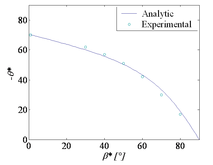
The prediction of the kink angle (\ref{eq:kinkangle}) is in good agreement with the experimental results obtained by Erdogan & Sih (1963), as shown on Picture V.15.
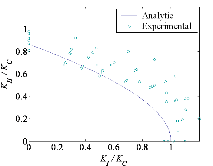
The resolution of this system of 2 equations (\ref{eq:beta}) and (\ref{eq:KCMixed}) with 2 unknowns $K_I$ and $K_{II}$ leads to the failure envelope illustrated in Picture V.16. Toughness tests for different loading directions provide comparisons points reported in Picture V.16. On this figure it can be seen that the failure criterion (\ref{eq:KCMixed}) is conservative.
Pure mode II loading
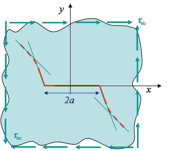
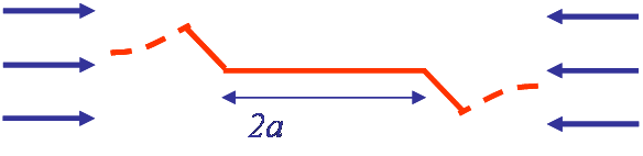
The pure mode II loading is characterized by $\beta^\star = 0$ as $K_I = 0$. Note that this case cannot be represented by a tension oriented with $\beta^\star=0$ as in Picture V.13, as in this case the crack is not loaded. The correct representation is shown in Picture V.17. Nevertheless the maximum hoop stress theory can be applied to this case because of the general definition of $\beta^\star$ (\ref{eq:beta}). The kink angle can be directly deduced from Picture V.15, and the threshold on $K_{II}$ before crack growth from Picture V.16. These values can also be computed in a closed form as follows.
-
The kink angle is obtained from (\ref{eq:kinkangle}) with $\beta^\star = 0$, leading to
\begin{equation} \tan{\frac{\theta^\star}{2}} = -\sqrt{\frac{1}{2}}\quad \iff \theta^\star|_{\beta^\star = 0} \approx -70.53\text{°}.\label{eq:kinkModeII} \end{equation} -
The failure threshold on $K_{II}$ can be obtained from (\ref{eq:KCMixed1}) using (\ref{eq:kinkModeII}), leading to
\begin{eqnarray} \frac{K_{II}}{K_{IC}}&=&-\frac{1}{3\sin{\frac{\theta}{2}}\cos^2{\frac{\theta}{2}}}= -\frac{\left(1+\tan^2{\frac{\theta}{2}}\right)^\frac{3}{2}} {3\tan{\frac{\theta}{2}}} = \sqrt{\frac{3}{4}}\nonumber\\ \iff K_{II} &\simeq& 0.87 K_{IC}.\label{eq:KCModeII}\end{eqnarray}
From this last results it appears that the critical value of the SIF in mode II loading is lower than the mode I toughness.
Let us now compare these predictions with an engineering judgment. For a plate under shearing, the circumferential stress reads
\begin{equation} \mathbf{\sigma}_{\theta\theta}= - \tau_\infty \sin{2\theta}, \end{equation}
which is maximum for $\theta = -45$°. One could thus expect the crack to propagate along this $-45$° shear-plane direction while the theory predicts a kink angle $\theta^\star|_{\beta^\star = 0}\neq -45$°. This discrepancy is even more worrying as experimentally cracks are observed to propagate with a -$45$°-angle. How can we explain this difference? We have develop the theory using the asymptotic solution and found that due to the stress field resulting from the presence of the crack, the maximum circumferential stress at crack tip is obtained for $\theta = -70.53$°. The crack thus kinks with this angle. As it grows, the crack does not remain under pure mode II loading and the new stress distribution at the crack tip makes it turn until growing with a pure -45°-angle so that is sees a pure mode I loading, as illustrated by Picture V.18.
Remember that when using the asymptotic solution (\ref{eq:asympModeII}) we have only considered the dominant term in $\frac{1}{\sqrt{r}}$. We can also consider the next term in the series in $r^0$, which is a constant term, when interested to know what happen at distance $r_c$ from the crack tip. For a plate in shearing, it has been shown that such a second order theory predicts a kink angle which reduces as the crack propagates.
Second order theory
As said, we have only considered the dominant term in $\frac{1}{\sqrt{r}}$ of the asymptotic solution. When analyzing the behavior at a distance $r_c$ from the crack tip, we need to include the next term in the series in $r^0$, which is a constant term. Let us considered the mixed mode loading characterized by a ratio $\beta^\star$ (\ref{eq:beta}) as before, but this time we consider the higher order term under the form of a constant traction $T$ along the $x$-axis, see Picture V.19. Then the hoop stress (\ref{eq:hoop}) becomes
\begin{eqnarray} &\mathbf{\sigma}_{\theta\theta}\left(r_c,\theta\right)=\nonumber\\& \frac{K_I}{\sqrt{2\pi r_c}}\left[\cos^3{\frac{\theta}{2}}-\frac{3\cot{\beta^*}}{2}\sin{\theta}\cos{\frac{\theta}{2}}\right]+T\sin^2{\theta}.\label{eq:hoopHigherTerm} \end{eqnarray}
While the asymptotic solution is solely characterized by the SIFs, this high order theory predicts a new kink angle $\theta^\star(\beta^\star,\, T,\, r_c,\, K_I)$ which depends on the stress field at a distance $r_c$, where $r_c$ is determined by experiments (for Aluminum alloys $r_c\simeq 1.5$ mm) .
This method can be used in FE simulation, and the results obtained numerically for a mixed mode loading can be summarized as follows
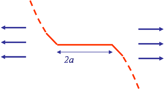
- For compression ($T< 0$), see Picture V.20, or low traction after the initial kink predicted by the asymptotic solution, the crack tends to align itself with $T$.
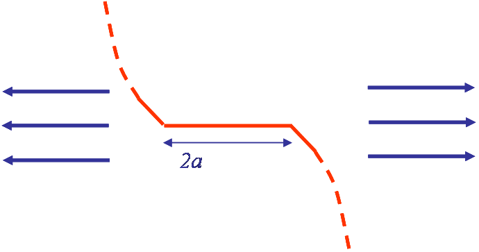
- For traction of the order of $\frac{K_I}{\sqrt{r}}$, see Picture V.21, or larger, see Picture V.22, there is bifurcation and the crack tends to become perpendicular to $T$.
Method of maximum energy release rate
We have developed a theory based on the assumption that the crack propagates in a direction that maximizes the hoop stress. Another possible assumption is based on thermodynamics considerations: equilibrium corresponds to the lowest potential energy so that the crack propagates to minimize the system potential energy. As the energy release rate is defined by $G = -\partial_A (E_\text{int} - W_\text{ext}) = -\partial_A \Pi_T$, this assumption corresponds to state that the crack grows in the direction maximizing $G$.
Methodology

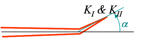
Let us consider a crack tip under mixed mode loading, with the SIFs at crack tip before crack propagation denoted by $k_I$ and $k_{II}$, see Picture V.23. This mixed loading is characterized by an angle $\beta^\star$ such that $\cot \beta^\star = \frac{k_{II}}{k_I}$. We assume that under this mixed loading conditions, the crack propagates and forms a kink of infinitesimal length and of angle $\alpha$. Because of the kink propagation the stress field changes and the we have new SIFs at the crack tip just after the kink propagation, which are denoted $K_I$ and $K_{II}$, see Picture V.24. The new $K_i(\alpha)$ can be deduced from the former $k_i$ following the first order (in $\alpha$) accurate relation found by Cotterell & Rice (1980):
\begin{equation}
\left(\begin{array}{c}
K_{I}\left(\alpha\right)\\
K_{II}\left(\alpha\right)
\end{array}\right)
=\frac{1}{4}\left(\begin{array}{cc}
3\cos{\frac{\alpha}{2}}+\cos{\frac{3\alpha}{2}} & -3\sin{\frac{\alpha}{2}}-3\sin{\frac{3\alpha}{2}} \\
\sin{\frac{\alpha}{2}}+\sin{\frac{3\alpha}{2}} & \cos{\frac{\alpha}{2}}+3\cos{\frac{3\alpha}{2}}
\end{array}\right)
\left(
\begin{array}{c}
k_I\\
k_{II}
\end{array}\right).\label{eq:CotterellRice}
\end{equation}
In linear elasticity, as the kink grows straight ahead we can use the relation between the energy release rate and the SIFs related to the kink (not the ones related to the initial crack as this one does not grow straight ahead), leading to
\begin{equation} G=\frac{K^2_I\left(\alpha\right)+K^2_{II}\left(\alpha\right)}{E'} = f\left(k_I,\,k_{II},\,\alpha\right).\label{eq:Gkink} \end{equation}
Thus the potential kink direction $\alpha^\star$ is obtained by seeking for the extremum of this relation with respect to $\alpha$ and the fracture criterion is obtained by considering the energy release rate for a growth following that direction:
\begin{equation}\begin{cases} \left.G_{,\alpha}\right|_{\alpha^\star}=0 \text{ with } \left.G_{,\alpha\alpha}\right|_{\alpha^\star}<0 \\ G\left(\alpha^\star\right)\geq G_C \end{cases}.\label{eq:maxG}\end{equation}
Results
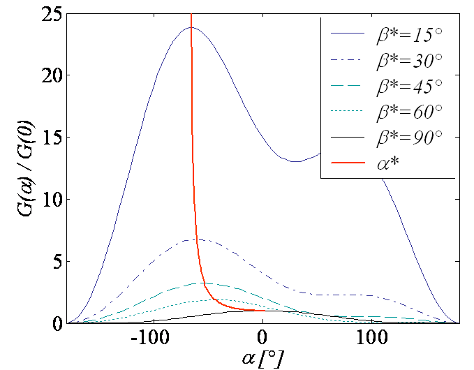
Picture V.25 illustrates the evolution of the energy release rate after kink propagation obtained from (\ref{eq:CotterellRice} - \ref{eq:Gkink}) for different values of $\beta^\star$ such that $\cot \beta^\star = \frac{k_{II}}{k_I}$. The blue curve is the maximum locus obtained by resolving the system (\ref{eq:CotterellRice} - \ref{eq:maxG}) and corresponds to the kink angle leading to the maximum energy release rate. As for the method of the maximum hoop stress, the kink angle is found to be negative for positive loading angles.
Note that we used a formula accurate only to the first order in $\alpha$, which leads to an error on the resolution:
- $ < 5$% error for $\alpha < 40$°;
- $\approx 5$% error on $K_I$ for $\alpha > 40$° (Cotterell & Rice, 1980).
Comparison of the methods
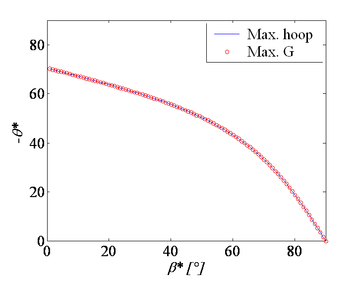
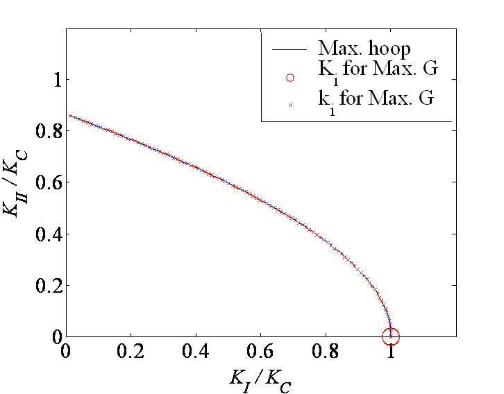
We have predicted the kink angle using the maximum hoop stress method (\ref{eq:kinkangle}) and using the maximum energy release rate method (\ref{eq:maxG}). As it can be seen on Picture V.26, both methods lead to similar kink angles for the same mixed loading conditions. We can also compare the failure envelope, meaning the combination of SIFs before crack growth, leading to fracture. With the maximum energy release rate method this envelope is thus in terms of $k_I$ and $k_{II}$. One more time as it can be seen in Picture V.27 both methods give the same predictions. Note that when using the maximum energy release rate method, one can obtain the SIF after crack kink from (\ref{eq:CotterellRice}). As shown in Picture V.27 this method predicts a mode I SIF related to the kink equal to $K_C$ while the mode II SIF vanishes. This demonstrates that the crack kinks in a direction so that ii becomes loaded in pure mode I, maximizing the energy release rate in the same time.
We have considered crack growth due to static loading. However for cyclic loading we can have crack growth while the SIFs remain much lower than the toughness. The next page talks about fatigue failure.
![]()