
Cohesive Zone > Cohesive Zone Models
Introduction to the Cohesive Zone Models (CZMs)
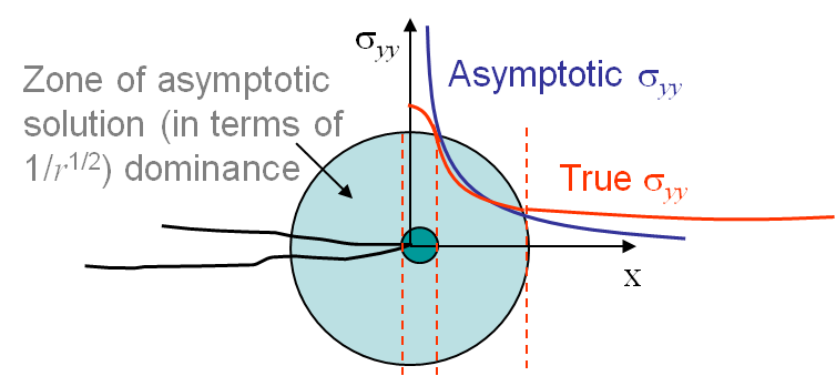
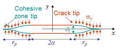
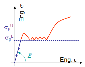
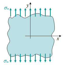
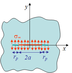
The idea behind the cohesive zone models is to remove the stress singularity of the asymptotic solution, see Picture VII.5, by introducing a plastic zone at the crack tip, see Picture VII.6. The cohesive zone models assume that the nonlinearities are localized at the crack tip, in the so-called process zone which extends on a length $r_p$ ahead of crack tip, see Picture VII.6. The opening of the crack at crack tip is thus non-zero and is referred to as the Crack Tip Opening Displacement (CTOD) $\delta_t$. The two main Cohesive Zone Models are now introduced.
Dugdale's Cohesive Zone/Yield Strip Model
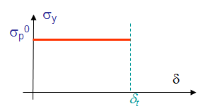
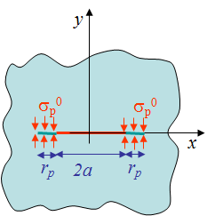
Dugdale's model assumes that the material is elastic-perfectly plastic, that is, the material of the specimen under consideration yields with minimal or zero strain hardening. As a result, the stress $\sigma_y$ in the process zone is uniform for all process zone opening $\delta$ until reaching the crack tip opening displacement $\delta_t$. This stress corresponds to the initial yield stress of the material $\sigma_p^0$ as illustrated in Picture VII.7.
Dugdale's model is valid
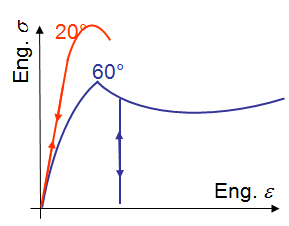
- For glassy polymers such as PVC, Plexiglas under ductile to brittle transition temperature, see Picture VII.8;
- For thin sheets made of elastic-perfectly plastic materials;
- For low carbon steels exhibiting Lüders' bands where dislocations motion is initially blocked by solute atoms and once freed leads to a decrease of the yielding point, see Picture VII.9; An illustration of the Lüders' bands can be seen in Picture VII.10.
Barenblatt's Cohesive Model
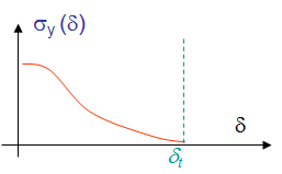
Barenblattt's model represents the decrease of the atomic or molecular attraction with the increase of the separation $\delta$, until vanishing at the CTOD $\delta_t$, see Picture VII.11. This model also allows avoiding the stress singularity at the crack tip. Moreover, the fracture response is uniquely governed by the shape of the decreasing curve. However, as the model is directly related to the evolution of the bonding between atoms, this model is valid only for brittle materials.
Description of Dugdale's model
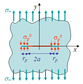
Dugdale has developed a model in which the process zone is subjected to a constant surface traction corresponding to the yield stress $\sigma_p^0$, see Picture VII.7 and Picture VII.12. Since the non-linearities are limited in the process zone and are replaced by boundary conditions, the problem can be solved using LEFM. The length of the cohesive zone $r_p$ is then defined in order to remove the stress singularity inherent to LEFM.
Since LEFM is used for solving this problem, the superposition principle holds and the solution of the problem illustrated in Picture VII.12 is the superposition of the three cases shown in Picture VII.13 to Picture VII.15. After having recalled the main ingredients to solve linear elasticity in a cracked plate, the three cases are successively solved.
LEFM resolution using Westergaard functions
Under the assumptions of 2D linear elasticity, the problem can be stated in terms of the Airy function and is thus governed by the bi-harmonic equation:
\begin{equation} \nabla^2 \nabla^2 \Phi = 0 .\label{eq:biharmonic}\end{equation}
One solution of this equation has the form:
\begin{equation} \Phi = \frac{\bar{\zeta}\Omega+\zeta\bar{\Omega} + \omega + \bar{\omega}}{2} ,\label{eq:PhiCrack}\end{equation}
where the functions $\omega(\zeta)$ and $\Omega(\zeta)$ have to be determined so that the boundary conditions are satisfied. The solution fields can be expressed in terms of these functions as follows:
- The stress field reads: \begin{equation} \left\{ \begin{array}{r c l} \mathbf{\sigma}_{xx} &= &\Omega'+\bar{\Omega}' - \frac{\bar{\zeta}\Omega''+\omega''+ \zeta\bar{\Omega}''+ \bar{\omega}''}{2},\\ \mathbf{\sigma}_{yy} &=&\Omega'+\bar{\Omega}' + \frac{\bar{\zeta}\Omega''+\omega''+ \zeta\bar{\Omega}''+ \bar{\omega}''}{2},\\ \mathbf{\sigma}_{xy} &=& i \frac{\zeta\bar{\Omega}''+\bar{\omega}''-\bar{\zeta}\Omega''-\omega''}{2}. \end{array} \right. \label{eq:stressAiry}\end{equation}
- The displacement field reads: \begin{equation} \mathbf{u} = -\frac{1+\nu}{E}\left(\zeta\bar{\Omega}'+\bar{\omega}' + \kappa \left(\zeta\right)\right),\label{eq:uAiry} \end{equation} with \begin{equation} \left\{ \begin{array}{r c l l} \kappa &=&\frac{3-\nu}{1+\nu}&\text{ in Plane} \quad \sigma,\\ \kappa &=&3-4\nu&\text{ in Plane} \quad\epsilon. \end{array} \right. \label{eq:kappaAiry}\end{equation}
The resolution of a loaded crack can be found using the Westergaard functions as detailed in the SIF lecture. For a mode I loading, see Picture VII.16, the choice $\omega''=-\zeta\Omega''$ leads to cancel the shear stress $\mathbf{\sigma}_{xy}$ along the $x$-axis as shown in the SIF lecture. Indeed, the stress (\ref{eq:stressAiry}) and displacement fields (\ref{eq:uAiry}) become, see details in the SIF lecture, respectively
\begin{equation} \left\{ \begin{array}{r c l} \mathbf{\sigma}_{xx} &=& 2\mathcal{R}\left(\Omega'\right)-2 y\mathcal{I}\left(\Omega''\right),\\ \mathbf{\sigma}_{yy} &=& 2\mathcal{R}\left(\Omega'\right)+2 y\mathcal{I}\left(\Omega''\right),\\ \mathbf{\sigma}_{xy} &=& -y2\mathcal{R}\left(\Omega''\right),\text{ and}\\ \mathbf{u}_x &=& \mathcal{R}\left(\mathbf{u}\right) = \frac{1+\nu}{E}\left[\left(\kappa-1\right)\mathcal{R}\left(\Omega\right)-2y\mathcal{I}\left(\Omega'\right)\right],\\ \mathbf{u}_y &=& \mathcal{I}\left(\mathbf{u}\right) = \frac{1+\nu}{E}\left[\left(\kappa+1\right)\mathcal{I}\left(\Omega\right)-2y\mathcal{R}\left(\Omega'\right)\right]. \end{array} \right.\label{eq:WeestMode1}\end{equation}
At this level only $\Omega$ has to be defined so that the stress and displacement fields satisfy the boundary conditions shown in Picture VII.16.
Resolution of Case 1
The solution of the first case, see Picture VII.17, is directly obtained using elasticity theory following the derivation in the SIF lecture:
\begin{equation} \left. \begin{array}{l c l} \mathbf{\sigma}_{yy}&=&\mathbf{\sigma}_\infty\\ \mathbf{\sigma}_{xx}&=&\mathbf{\sigma}_{xy}=0\end{array}\right\}\Longrightarrow\left\{ \begin{array}{ r c l} \epsilon_{xx}& = &\frac{\left(1+\nu\right)\left(3-\kappa\right)}{4E}\mathbf{\sigma}_\infty\,,\\ \epsilon_{yy}& =& \frac{\left(1+\nu\right)\left(1+\kappa\right)}{4E}\mathbf{\sigma}_\infty\,,\\ \epsilon_{xy}& =& 0\,,\\ u_{x} &=&\frac{\left(1+\nu\right)\left(3-\kappa\right)}{4E}\mathbf{\sigma}_\infty x\,,\\ u_{y} &=&\frac{\left(1+\nu\right)\left(1+\kappa\right)}{4E}\mathbf{\sigma}_\infty y\,.\\ \end{array}\right. \label{eq:SIFcase1} \end{equation}
Resolution of Case 2
A similar problem as the second case, Picture VII.18, has been solved in the SIF lecture, but for a different crack length, and the solution is directly obtained by substituting $a$ by $a+r_p$
\begin{equation} \left\{\begin{array}{l c l} \Omega&=&\frac{\mathbf{\sigma}_\mathbf{\infty}}{2}\bigg(\sqrt{\mathbf{\zeta}^2-{\left(a+r_p\right)}^2}-\mathbf{\zeta}\bigg)\,,\\ \Omega'&=&\frac{\mathbf{\sigma}_\mathbf{\infty}}{2}\bigg(\frac{\mathbf{\zeta}}{\sqrt{\mathbf{\zeta}^2-{\left(a+r_p\right)}^2}}-1\bigg)\,,\\ \Omega''&=&-\frac{\mathbf{\sigma}_\mathbf{\infty}}{2}\bigg(\frac{(a+r_p)^2}{\sqrt{\mathbf{\zeta}^2-{\left(a+r_p\right)}^2}^3}\bigg)\,.\\ \end{array}\right. \label{eq:OmegaCase2}\end{equation}
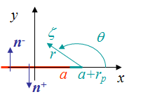
Therefore, considering the polar coordinates linked to the end of the process zone, Picture VII.19, the stress field ahead of the cohesive zone tip follows from the same argumentation as in the SIF lecture, leading to:
\begin{equation} \left\{\begin{array}{l c l} \mathbf{\sigma}_{xy}\left(\mathbf{\theta}=0\right)&=&0\,,\\ \mathbf{\sigma}_{xx}\left(\mathbf{\theta}=0\right)&=&2\mathcal{R}\left(\mathbf{\Omega}'\right)=\mathbf{\sigma}_\mathbf{\infty}\bigg(\frac{x}{\sqrt{x^2-{\left(a+r_p\right)}^2}}-1\bigg)\,,\\ \mathbf{\sigma}_{yy}\left(\mathbf{\theta}=0\right)&=&2\mathcal{R}\left(\mathbf{\Omega}'\right)=\mathbf{\sigma}_\mathbf{\infty}\bigg(\frac{x}{\sqrt{x^2-{\left(a+r_p\right)}^2}}-1\bigg)\,,\\\end{array}\right. \label{eq:SIFCase2}\end{equation}
and the displacement field of the crack lips and process zone also follows from the same argumentation as in the SIF lecture, leading to:
\begin{equation} \lim_{\theta\rightarrow\pm\pi} u_y =\pm \frac{\left(1+\nu\right)\left(\kappa+1\right)\sigma_\infty} {2E} \sqrt{\left(a+r_p\right)^2-x^2} \,.\label{eq:uCase2}\end{equation}
Resolution of Case 3
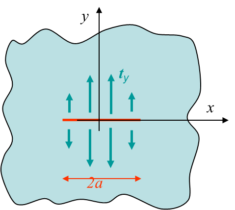
The resolution of the third case is stated as finding $\Omega$ so that the boundary conditions illustrated on see Picture VII.20 are satisfied, i.e. such that
- The crack lips $(|x| < a)$ are stress-free, which is rewritten using Eq. (\ref{eq:WeestMode1}) for respectively the upper ($\theta\rightarrow +\pi$) and lower ($\theta\rightarrow -\pi$) lips as \begin{equation} \mathbf{t}(\theta\rightarrow \pm\pi)=\mathbf{\sigma}\cdot\mathbf{n}=\mp\mathbf{\sigma}_{yy}=\mp2\mathcal{R}\Omega'=0\,;\label{eq:case3cracklips} \end{equation}
- The processe zone $(a<| x |< a+r_p)$ is subjected to the surface pressue $-\sigma_p^0$, which is rewritten using Eq. (\ref{eq:WeestMode1}) for respectively the upper ($\theta\rightarrow +\pi$) and lower ($\theta\rightarrow -\pi$) lips as \begin{equation} \mathbf{t}(\theta\rightarrow \pm \pi)=\mathbf{\sigma}\cdot\mathbf{n}=\mp\mathbf{\sigma}_{yy}=\mp2\mathcal{R}\Omega'=\mp\sigma_p^0\,;\label{eq:case3cohesivezone}\end{equation}
- In addition, the plate should be stress free at positions far away from the crack.
Considering the right part of the sample ($x\geq0$), and using the complex referential represented in Picture VII.19, the solution $\Omega$ which satisfies these conditions is
\begin{equation} \left\{\begin{array}{rcl} \Omega &=&-\frac{\sigma_p^0}{\pi}\sqrt{\mathbf{\zeta}^2-{\left(a+r_p\right)}^2}\text{arcotan}\frac{a}{\sqrt{r_p^2+2ar_p}}-\frac{\sigma_p^0a}{\pi}\text{arcotan}\sqrt{\frac{\mathbf{\zeta}^2-{\left(a+r_p\right)}^2}{r_p^2+2ar_p}}+\\&&\frac{\sigma_p^0\mathbf{\zeta}}{\pi}\text{arcotan}\bigg(\frac{a}{\mathbf{\zeta}}\sqrt{\frac{\mathbf{\zeta}^2-{\left(a+r_p\right)}^2}{r_p^2+2ar_p}}\bigg)\,, \\ \Omega'&=&-\frac{\sigma_p^0}{\pi}\frac{\mathbf{\zeta}}{\sqrt{\mathbf{\zeta}^2-{\left(a+r_p\right)}^2}}\text{arcotan}\frac{a}{\sqrt{r_p^2+2ar_p}}+\frac{\sigma_p^0}{\pi}\text{arcotan}\bigg({\frac{a}{\mathbf{\zeta}}\sqrt{\frac{\mathbf{\zeta}^2-{\left(a+r_p\right)}^2}{r_p^2+2ar_p}}}\bigg)\,,\end{array}\right.\label{eq:OmegaPrimCase3}\end{equation}
as it will be shown here below. The derivative $\Omega'$ is obtained from $\Omega$ using the identity $d_{\mathbf{\zeta}} \text{arcotan} \mathbf{\zeta} = -\frac{1}{1+\mathbf{\zeta}^2}$.
To demonstrate that Eq. (\ref{eq:OmegaPrimCase3}) is the solution of the third problem, it is first necessary to show that this function induces two discontinuities, one between the crack lips and the cohesive zone, and one between the cohesive zone and the sound material. Then the verification of the boundary conditions can be assessed.
- For $y=0$, ahead of the cohesive zone one has $x > a+r_p$ and $\sqrt{\mathbf{\zeta}^2-{\left(a+r_p\right)}^2}$ is a real number so that $\Omega'$ of Eq. (\ref{eq:OmegaPrimCase3}) is purely real.
- For $y=0$, on the crack lips and on the process zone, one has $0<x < a+r_p$ and $\sqrt{\mathbf{\zeta}^2-{\left(a+r_p\right)}^2}$ is no longer a real number. Using the identity $\text{arcotan}\,\mathbf{\zeta}=\frac{i}{2}\ln\frac{\mathbf{\zeta}-i}{\mathbf{\zeta}+i}$, the function (\ref{eq:OmegaPrimCase3}) is thus rewritten
\begin{equation}
\Omega'=\frac{-\sigma_p^0}{\pi}\frac{\mathbf{\zeta}}{\sqrt{\mathbf{\zeta}^2-{\left(a+r_p\right)}^2}}\text{arcotan}\frac{a}{\sqrt{r_p^2+2ar_p}}+\frac{i\sigma_p^0}{2\pi}\ln\frac{\frac{a}{\mathbf{\zeta}}\sqrt{\frac{\mathbf{\zeta}^2-{\left(a+r_p\right)}^2}{r_p^2+2ar_p}}-i}{\frac{a}{\mathbf{\zeta}}\sqrt{\frac{\mathbf{\zeta}^2-{\left(a+r_p\right)}^2}{r_p^2+2ar_p}}+i}
\,.\label{eq:OmegaPrimLnCase3}\end{equation} Considering the referential illustrated in Picture VII.19, for $\mathbf{\zeta}=x\pm i |\varepsilon|$, with $0<x<{a+r_p}$ and $\varepsilon\rightarrow 0$, we have \begin{equation}
\lim_{\theta\rightarrow\pm\pi} \sqrt{\mathbf{\zeta}-a-r_p}=\sqrt{r} \exp{\left(\pm\frac{i\pi}{2}\right)}=\pm{i}\sqrt{r}=\pm{i}\sqrt{a+r_p-x}\,,\end{equation} and Eq. (\ref{eq:OmegaPrimLnCase3}) is rewritten
\begin{equation}
\Omega'\left(\theta\rightarrow\pm\pi\right)=\pm{i}\frac{\sigma_p^0}{\pi}\frac{x}{\sqrt{{\left(a+r_p\right)}^2-x^2}}\text{arcotan}\frac{a}{\sqrt{r_p^2+2ar_p}}+\frac{{i}\sigma_p^0}{2\pi}\ln\frac{\pm\frac{a}{x}
\sqrt{\frac{{\left(a+r_p\right)}^2-{x^2}}{r_p^2+2ar_p}}-1}{\pm\frac{a}{x}\sqrt{\frac{{\left(a+r_p\right)}^2-{x^2}}{r_p^2+2ar_p}}+1}\,,
\label{eq:OmegaPrimLnTmpCase3}\end{equation} or again \begin{equation}\begin{array}{ll}
{\Omega'}\left(\theta\rightarrow\pm\pi\right) =& \pm i\frac{\mathbf{\sigma}_p^0}{\pi}\frac{x}
{\sqrt{\left(a+r_p\right)^2-x^2}}\text{arcotan} \frac{a}{\sqrt{r_p^2+2ar_p}}\pm \frac{i\mathbf{\sigma}_p^0}{2\pi} \ln\bigg( a\sqrt{\frac{\left(a+r_p\right)^2-x^2}{r_p^2+2ar_p}} -x\bigg)\mp\\
&\frac{i\mathbf{\sigma}_p^0}{2\pi}\ln\bigg(a\sqrt{\frac{\left(a+r_p\right)^2-x^2}{r_p^2+2ar_p}}+x\bigg)\,.\end{array}
\label{eq:OmegaPrimLnBisCase3}\end{equation}
Two cases can now be considered.
- On the crack lips, one has $0<x<a$, and $\frac{a}{x} \sqrt{\frac{{\left(a+r_p\right)}^2-{x^2}}{r_p^2+2ar_p}}=\frac{a}{x} \sqrt{\frac{r_p^2+2ar_p+\left(a^2-x^2\right)}{r_p^2+2ar_p}}>1$, and $\ln\left( a \sqrt{\frac{{\left(a+r_p\right)}^2-{x^2}}{r_p^2+2ar_p}}-x\right)$ yields a real number. As a result Eq. (\ref{eq:OmegaPrimLnBisCase3}) yields \begin{equation} \mathcal{R}\Omega'\left(0<x<a,\,\theta\rightarrow\pi\right) = 0,\, \end{equation} and Eq. (\ref{eq:case3cracklips}) is satisfied.
- On the process zone, one has $a<x<a+r_p$, and $\frac{a}{x} \sqrt{\frac{{\left(a+r_p\right)}^2-{x^2}}{r_p^2+2ar_p}}=\frac{a}{x} \sqrt{\frac{r_p^2+2ar_p+\left(a^2-x^2\right)}{r_p^2+2ar_p}}<1$, and $\ln\left(a \sqrt{\frac{{\left(a+r_p\right)}^2-{x^2}}{r_p^2+2ar_p}}-x\right)$ does not yield a real number. Using the identity $\ln z = \ln|z|+{i} \text{arg}{z}$ and since $\text{arg}\bigg(a\sqrt{\frac{\left(a+r_p\right)^2-\zeta^2}{r_p^2+2ar_p}}-\zeta\bigg) = -\pi$, Eq. (\ref{eq:OmegaPrimLnBisCase3}) becomes \begin{equation}\begin{array}{ll} {\Omega'}\left(\theta\rightarrow\pm\pi\right) =& \pm i\frac{\mathbf{\sigma}_p^0}{\pi}\frac{x} {\sqrt{\left(a+r_p\right)^2-x^2}}\text{arcotan} \frac{a}{\sqrt{r_p^2+2ar_p}}\pm \frac{\mathbf{\sigma}_p^0}{2} \pm \frac{i\mathbf{\sigma}_p^0}{2\pi} \ln\bigg( x- a\sqrt{\frac{\left(a+r_p\right)^2-x^2}{r_p^2+2ar_p}}\bigg)\mp\\ &\frac{i\mathbf{\sigma}_p^0}{2\pi}\ln\bigg(a\sqrt{\frac{\left(a+r_p\right)^2-x^2}{r_p^2+2ar_p}}+x\bigg)\,.\end{array} \label{eq:OmegaPrimLnCohCase3}\end{equation} As a result Eq. (\ref{eq:OmegaPrimLnCohCase3}) yields \begin{equation} \mathcal{R}\Omega'\left(a<x<a+r_p,\,\theta\rightarrow\pi\right) = \pm\frac{\sigma_p^0}{2},\, \end{equation} and Eq. (\ref{eq:case3cohesivezone}) is satisfied.
- Moreover, far away from the crack, one has \begin{equation} \lim_{\zeta\rightarrow\infty} \Omega' = -\frac{\sigma_p^0}{\pi}\text{arcotan}\frac{a}{\sqrt{r_p^2+2ar_p}}+\frac{\sigma_p^0}{\pi}\text{arcotan}\frac{a}{\sqrt{r_p^2+2ar_p}}=0\,, \end{equation} and \begin{equation} \lim_{|\zeta|\rightarrow\infty} \Omega'' = 0\,, \end{equation} so that $\mathbf{\sigma}_{xx} \left(\zeta\rightarrow\infty\right)\rightarrow {0} $ and $ \mathbf{\sigma}_{yy}\left(\zeta\rightarrow\infty\right)\rightarrow {0}$ are satisfied.
- Finally, for $x=0$, one has \begin{equation} \begin{array}{rcl} \Omega\left(x = 0\right)&=& \mp \frac{\sigma_p^0 i}{\pi} \sqrt{y^2+\left(a+r_p\right)^2} \text{arcotan} \frac{a}{\sqrt{r_p^2+2ar_p}} - \frac{\sigma_p^0{a}}{\pi} \text{arcotan} \left( \pm{i} \sqrt{\frac{y^2+{\left(a+r_p\right)}^2}{r_p^2+2ar_p}}\right) +\\&& \frac{\sigma_p^0iy}{\pi} \text{arcotan} \left(\pm\frac{a}{y}\sqrt{\frac{y^2+\left(a+r_p\right)^2}{r_p^2+2ar_p}}\right)\,,\\ \Omega'\left(x = 0\right)&=&\frac{\pm\sigma_p^0}{\pi}\frac{y}{\sqrt{y^2+\left(a+r_p\right)^2}}\text{arcotan}\frac{a}{\sqrt{r_p^2+2ar_p}}+\frac{\sigma_p^0}{\pi} \text{arcotan} \left(\pm\frac{a}{y}\sqrt{\frac{y^2+\left(a+r_p\right)^2}{r_p^2+2ar_p}}\right)\,.\end{array}\label{eq:case3x0}\end{equation} As a result $\mathcal{R}\left(\Omega\right) = 0$ and $\mathcal{I}\left(\Omega'\right) = 0 $ so that using Eq. (\ref{eq:WeestMode1}), $\mathbf{u}_x\left(x=0\right) = 0$ is satisfied.
We can now evaluate the stress field ahead of the cohesive zone. For $\mathbf{\zeta} = x \pm|\varepsilon| i$, with $\varepsilon\rightarrow 0$ and $a+r_p < x$, Eq. (\ref{eq:OmegaPrimCase3}) is rewritten
\begin{equation} \Omega'=-\frac{\sigma_p^0}{\pi}\frac{x}{\sqrt{x^2-{\left(a+r_p\right)}^2}}\text{arcotan}\frac{a}{\sqrt{r_p^2+2ar_p}}+\frac{\sigma_p^0}{\pi}\text{arcotan}\left(\frac{a}{x}\sqrt{\frac{x^2-{\left(a+r_p\right)}^2}{r_p^2+2ar_p}}\right) \,, \label{eq:OmegaPrimCase3theta0}\end{equation}
and the stress field ahead of the cohesive zone is given from Eq. (\ref{eq:WeestMode1}) as,
\begin{equation}\begin{array}{rcl} \mathbf{\sigma}_{yy}\left(\theta=0\right)=2\mathcal{R}\Omega'\left(\theta=0\right)&=&-\frac{2\sigma_p^0}{\mathbf{\pi}}\frac{x}{\sqrt{x^2-{\left(a+r_p\right)}^2}}\text{arcotan}\frac{a}{\sqrt{r_p^2+2ar_p}}+\\&&\frac{2\sigma_p^0}{\pi}\text{arcotan}\left(\frac{a}{x}\sqrt{\frac{x^2-{\left(a+r_p\right)}^2}{r_p^2+2ar_p}}\right)\,.\end{array}\label{eq:SIFCase3} \end{equation}
The displacement field on the crack lips and on the cohesive zone can be obtained by rewriting Eq. (\ref{eq:OmegaPrimCase3}) for $\mathbf{\zeta} = x \pm|\varepsilon| i$, with $\varepsilon\rightarrow 0$ and $0 \leq x < a+r_p$, as
or again using the identity $\text{arcotan}\,\mathbf{\zeta}=\frac{i}{2}\ln\frac{\mathbf{\zeta}-i}{\mathbf{\zeta}+i}$, as
\begin{equation} \begin{array}{rcl} \Omega\left(\theta\rightarrow \pm \pi\right) &=& \mp \frac{\sigma_p^0 i }{\pi}\sqrt{\left(a+r_p\right)^2-x^2} \text{arcotan} \frac{a}{\sqrt{r_p^2+2ar_p}} \mp \frac{ \sigma _p^0 ai }{2\pi} \ln \left(\frac{ \sqrt{ \frac{\left(a+r_p\right)^2-x^2}{r_p^2+2ar_p}}-1} {\sqrt{\frac{\left(a+r_p\right)^2-x^2}{r_p^2+2ar_p}}+1}\right) \pm \\ && \frac{\sigma_p^0{xi}}{2\pi} \ln \frac{\frac{a}{x} \sqrt{ \frac{\left(a+r_p\right)^2-x^2}{r_p^2+2ar_p}}-1} {\frac{a}{x}\sqrt{\frac{\left(a+r_p\right)^2-x^2}{r_p^2+2ar_p}}+1} \,.\end{array}\label{eq:OmegaPrimCase3thetaLn}\end{equation}
We now need to consider separately the displacement fields on the crack lips and on the process zone:
- For $x<a$, i.e. on the crack lips, the arguments of the logarithm functions are real and using the identity $\text{arcoth} x = \frac{1}{2} \ln \frac{x+1}{x-1}$, Eq. (\ref{eq:OmegaPrimCase3thetaLn}) becomes \begin{equation} \begin{array}{rcl} \Omega\left(\theta\rightarrow \pm\pi\right) &=& \mp\frac{\sigma_p^0i}{\pi}\sqrt{\left(a+r_p\right)^2-x^2}\text{arcotan}\frac{a}{\sqrt{r_p^2+2ar_p}} \pm \frac{\sigma_p^0{ai}}{\pi}\text{arcoth}\sqrt{\frac{\left(a+r_p\right)^2-x^2}{r_p^2+2ar_p}} \mp\\ && \frac{\sigma_p^0{xi}}{\pi}\text{arcoth}\left(\frac{a}{x}\sqrt{\frac{\left(a+r_p\right)^2-x^2}{r_p^2+2ar_p}}\right)\,. \end{array} \label{eq:OmegaPrimCase3thetaPiCrackLips}\end{equation} The displacement field for $y=0$ and $x<a$ is then obtained using Eq. (\ref{eq:WeestMode1}) as \begin{equation}\begin{array}{rcl} u_y\left(\theta\rightarrow \pm \pi\right) &=& \pm \frac{\left(1+\nu\right)\left(1+\kappa\right) \sigma_p^0}{E\pi} \bigg[-\sqrt{\left(a+r_p\right)^2-x^2} \text{arcotan} \frac{a}{\sqrt{r_p^2+2ar_p}} + a \text{arcoth} \sqrt{ \frac{\left(a+r_p\right)^2 - x^2}{r_p^2 + 2ar_p}}\\ &&- x \text{arcoth} \left(\frac{a}{x}\sqrt{ \frac{\left(a+r_p\right)^2 - x^2}{r_p^2 + 2ar_p}}\right) \bigg]\,.\end{array} \label{eq:uCase3CrackLips}\end{equation}
- For $a<x<a+r_p$, i.e. on the process zone, the arguments of the second logarithm function is not real and using the identity $\ln{z} = \ln |z| + i \arg{z}$, Eq. (\ref{eq:OmegaPrimCase3thetaLn}) becomes \begin{equation} \begin{array}{rcl} \Omega\left(\theta\rightarrow \pm \pi\right) &=& \mp\frac{\sigma_p^0i}{\pi}\sqrt{\left(a+r_p\right)^2-x^2}\text{arcotan}\frac{a}{\sqrt{r_p^2+2ar_p}}\mp \frac{\sigma_p^0{ai}}{2\pi}\ln\left( \frac{\sqrt{ \frac{\left(a+r_p\right)^2-x^2}{r_p^2+2ar_p}}-1}{\sqrt{\frac{\left(a+r_p\right)^2-x^2}{r_p^2+2ar_p}}+1}\right) \pm\\&& \frac{\sigma_p^0x}{2}\pm\frac{\sigma_p^0{xi}}{2\pi} \ln \left( \frac{1-\frac{a}{x} \sqrt{ \frac{\left(a+r_p\right)^2-x^2}{r_p^2+2ar_p}}} {\frac{a}{x}\sqrt{\frac{\left(a+r_p\right)^2-x^2}{r_p^2+2ar_p}}+1}\right)\,,\end{array} \end{equation} or again using $\text{arctanh} x = \frac{1}{2} \ln \frac{x+1}{1-x}$ as \begin{equation}\begin{array}{rcl} \Omega\left(\theta\rightarrow\pm\pi\right) &=& \mp\frac{\sigma_p^0i}{\pi}\sqrt{\left(a+r_p\right)^2-x^2} \text{arcotan} \frac{a}{\sqrt{r_p^2+2ar_p}}\pm\frac{\sigma_p^0x}{2}\pm\frac{\sigma_p^0{ai}}{\pi} \text{arcoth} \sqrt{\frac{\left(a+r_p\right)^2-x^2}{r_p^2+2ar_p}}\mp\\&& \frac{\sigma_p^0{xi}}{\pi}\text{arctanh}\left(\frac{a}{x}\sqrt{\frac{\left(a+r_p\right)^2-x^2}{r_p^2+2ar_p}}\right)\,. \end{array} \label{eq:OmegaPrimCase3thetaPiCohesiveZone}\end{equation}The displacement field for $y=0$ and $x<a$ is then obtained using Eq. (\ref{eq:WeestMode1}) as \begin{equation}\begin{array}{rcl} u_y\left(\theta\rightarrow \pm \pi\right) &=& \pm \frac{\left(1+\nu\right)\left(1+\kappa\right) \sigma_p^0}{E\pi} \bigg[-\sqrt{\left(a+r_p\right)^2-x^2} \text{arcotan} \frac{a}{\sqrt{r_p^2+2ar_p}} + a \text{arcoth} \sqrt{ \frac{\left(a+r_p\right)^2 - x^2}{r_p^2 + 2ar_p}}\\ &&- x \text{arctanh} \left(\frac{a}{x}\sqrt{ \frac{\left(a+r_p\right)^2 - x^2}{r_p^2 + 2ar_p}}\right) \bigg]\,.\end{array} \label{eq:uCase3CohesiveZone}\end{equation}
By combining Eq. (\ref{eq:uCase3CrackLips}) and Eq. (\ref{eq:uCase3CohesiveZone}), the displacement field can be written as
\begin{equation}\begin{array}{rcl} u_y\left(\theta\rightarrow \pm \pi\right) &=& \pm \frac{\left(1+\nu\right)\left(1+\kappa\right) \sigma_p^0}{E\pi} \bigg[-\sqrt{\left(a+r_p\right)^2-x^2} \text{arcotan} \frac{a}{\sqrt{r_p^2+2ar_p}} + a \text{arcoth} \sqrt{ \frac{\left(a+r_p\right)^2 - x^2}{r_p^2 + 2ar_p}}\\ &&- x f\left(\frac{a}{x}\sqrt{ \frac{\left(a+r_p\right)^2 - x^2}{r_p^2 + 2ar_p}}\right) \bigg]\,,\end{array} \label{eq:uCase3}\end{equation}
where
\begin{equation}f(x) = \left\{\begin{array}{ll} \text{arcoth}(x) &\text{ if } x<a\, ;\\ \text{arctanh}(x) &\text{ if } a<x<a+r_p\,.\end{array}\right. \label{eq:fUCase3}\end{equation}
![]()