
SIF Computation > Experimental methods (LEMF)
Strain Gauge Method
The idea is similar to the correlation method used with FE analyzes. However in this case we extract the deformation field using a stain gauge, and then try to correlate the measures with the asymptotic solution. When considering a strain gauge, the question which arises is where to locate it? The asymptotic solution as developed before is only valid really close to the crack tip. Due to the size of the strain gauge it is not possible to mount it in such a small location. The asymptotic solution should thus account for higher order terms. Details on the method can be found in "Dally JW and Sanford RJ (1988), Strain gauge methods for measuring the opening mode stress intensity factor $K_I$, Experimental Mechanics 27, 381-388", and only the main steps are given here.
Let us go back the asymptotic solution for mode I:
\begin{equation}\begin{cases} \mathbf{\sigma}_{xx} &= & \sum_{\lambda}\left(\lambda+1\right) r^\lambda
\left[\left(2C_1-C_3\right)\cos{\left(\lambda\theta\right)} - C_1\lambda \cos{\left(\left(\lambda-2\right)\theta\right)}\right] \,;\\\mathbf{\sigma}_{yy} &= & \sum_{\lambda}\left(\lambda+1\right) r^\lambda \left[\left(2C_1+C_3\right)\cos{\left(\lambda\theta\right)} + C_1\lambda \cos{\left(\left(\lambda-2\right)\theta\right)}\right] \,;\\
\mathbf{\sigma}_{xy} &= & \sum_{\lambda}\left(\lambda+1\right) r^\lambda \left[ C_1\lambda \sin{\left(\left(\lambda-2\right)\theta\right)}+C_3 \sin{\left(\lambda\theta\right)} \right]\,,\end{cases} \label{eq:stressAiryModeI} \end{equation}
with $\lambda=-1/2,0,1/2,...$
The first order asymptotic solution in $r^{-1/2}$ cannot be matched accurately using a strain gauge. So we consider the third order solution, which can be expressed in the polar coordinates under the form
\begin{equation} \left( \begin{array}{c} \sigma_{rr}\\ \sigma_{\theta \theta}\\ \sigma_{r\theta} \end{array}\right) =\frac{K_I}{\sqrt{2\pi r}}\mathbf{f}_{-1/2}\left(\theta\right) + C_0 \mathbf{f}_{0}\left(\theta\right) + C_{1/2} \sqrt{r} \mathbf{f}_{1/2}\left(\theta\right)\,.\label{eq:3rdorder} \end{equation}
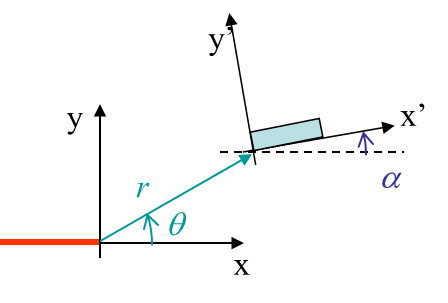
Remaining general, the strain gauge is located at the coordinates (r,$\theta$) linked to the crack tip, and with an orientation $\alpha$, see Picture IV.25. The third order asymptotic solution (\ref{eq:3rdorder}) leads to the expression of the measured strain:
\begin{equation}\begin{array}{ll} 2\mu \epsilon_{x'x'} &=& \frac{K_I}{\sqrt{2\pi r}} F\left(\nu,\, \theta,\,\alpha\right) +\\ &&C_0 \left(\frac{1-\nu}{1+\nu}+\cos{2\alpha}\right) + C_{1/2}\sqrt{r} \\&&\left(\frac{1-\nu}{1+\nu}+\sin^2{\frac{\theta}{2}}\cos{2\alpha} -\frac{1}{2}\sin\theta\sin{2\alpha}\right)\end{array}\,. \end{equation}
with
\begin{equation} F\left(\nu,\, \theta,\,\alpha\right) = \frac{1-\nu}{1+\nu}\cos{\frac{\theta}{2}} -\frac{1}{2}\sin{\theta}\sin{\frac{3\theta}{2}}\cos{2\alpha}+\frac{1}{2}\sin{\theta}\cos{\frac{3\theta}{2}}\sin{2\alpha} \,.\end{equation}
From these two expressions, one can see that by locating the strain gauge at (r,$\theta^*$, $\alpha^*$), such that
\begin{equation} \cos{2\alpha^*} = -\frac{1-\nu}{1+\nu} \text{ & } -\cot{2\alpha^*} = \tan{\frac{\theta^*}{2}}\,, \end{equation}
one can directly measure the SIF from
\begin{equation} K_I=\frac{2\mu \epsilon_{x'x'}\sqrt{2\pi r}}{ F\left(\nu,\, \theta^*,\,\alpha^*\right)}\,. \end{equation}
Remarks:
- Be aware that the mounting of the strain gauge is critical.
- Nowadays, the strain gauges are replaced by Digital Image Correlation (DIC).
![]()