
Asymptotic Solution > Resolution method based on Airy functions
The Airy functions
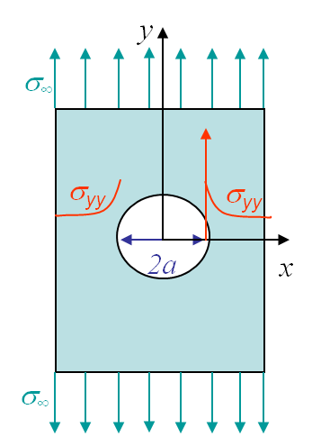
Before solving the problem of a cracked plate, we will explain the resolution method on typical mechanics problems as a plate with a circular, see Picture II.2, or elliptical, see Picture II.3, hole under tension. In this section we assume a static problem (no inertial forces). We will also consider the problem as being 2D, either in the plane stress state (P-$\sigma$) with
\begin{equation} \mathbf{\sigma}_{xz} = \mathbf{\sigma}_{yz} = \mathbf{\sigma}_{zz} = 0,\label{eq:planestress} \end{equation}
or in the plane strain state (P-$\varepsilon$) with
\begin{equation} \mathbf{\varepsilon}_{xz} = \mathbf{\varepsilon}_{yz} = \mathbf{\varepsilon}_{zz} = 0,\text{ and } \frac{\partial }{\partial z} = 0.\label{eq:planestrain} \end{equation}
In the following, Greek subscripts stand for x and y and Roman subscripts for x, y, and z. The Kronecker symbol is also used. Note that under these notations $\mathbf{\varepsilon}_{\alpha\alpha}=\mathbf{\varepsilon}_{xx}+\mathbf{\varepsilon}_{yy}$ and $\delta_{\alpha\alpha}=2$. Under the static assumption and assuming there is no volume forces $\mathbf{b}$, the linear momentum equation
\begin{equation} \rho \mathbf{\ddot{x}} = \nabla\cdot\mathbf{\sigma}^T + \mathbf{b}, \end{equation}
is simplified into
\begin{equation} \mathbf{\sigma}_{\alpha\beta,\beta} = 0 \label{eq:linearMomentumSimplified}, \end{equation}
where we have considered either (\ref{eq:planestress}) or (\ref{eq:planestrain}). Because of the particular form of (\ref{eq:linearMomentumSimplified}), there exists an Airy function so that
\begin{equation} \mathbf{\sigma}_{\alpha\beta} = -\Phi_{,\alpha\beta} + \delta_{\alpha\beta}\Phi_{,\gamma\gamma} \label{eq:Airy}. \end{equation}
Indeed the stress components (\ref{eq:Airy}) always satisfy (\ref{eq:linearMomentumSimplified}), as it is easily demonstrated by simple substitution of (\ref{eq:Airy}) into (\ref{eq:linearMomentumSimplified}). The meaning of this equation is particularly strong as one does not try anymore to solve the problem in terms of the stress tensor so that (\ref{eq:linearMomentumSimplified}) is satisfied, but one simply has to find a scalar function $\Phi$ from which the stress tensor derives following (\ref{eq:Airy}), knowing that (\ref{eq:linearMomentumSimplified}) is automatically satisfied.
The next step is to find the governing equation of $\Phi$. To do so, we consider the compatibility equation which is obtained by deriving (twice) $\mathbf{\varepsilon}_{xx}$ with respect to $yy$, deriving (twice) $\mathbf{\varepsilon}_{yy}$ with respect to $xx$ and deriving (twice) $\mathbf{\varepsilon}_{xy}$ with respect to $xy$. Using the definition of the strain components, one has directly the compatibility equation
\begin{equation} \mathbf{\varepsilon}_{xx,yy} +\mathbf{\varepsilon}_{yy,xx} = 2 \mathbf{\varepsilon}_{xy,xy} \label{eq:compatibility}.\end{equation}
These equations have been derived for both the P-$\sigma$ and P-$\varepsilon$ states. In order to relate the Airy function (and thus the stress tensor) to the compatibility equation (and thus to the strain tensor) we need to consider the material law whose expression differs in the P-$\sigma$ and P-$\varepsilon$ states.
Plane strain case
For the P-$\varepsilon$ state, the Hooke law combined with (\ref{eq:planestrain}) gives directly the stress components
\begin{equation} \begin{cases} \mathbf{\sigma}_{\alpha\beta} = \frac{E\nu}{\left(1+\nu\right)\left(1-2\nu\right)} \delta_{\alpha\beta} \mathbf{\varepsilon}_{\gamma\gamma} + \frac{E}{1+\nu}\mathbf{\varepsilon}_{\alpha\beta} \\ \mathbf{\sigma}_{zz} =\frac{E\nu}{\left(1+\nu\right)\left(1-2\nu\right)} \mathbf{\varepsilon}_{\gamma\gamma}
= \nu\mathbf{\sigma}_{\gamma\gamma} \end{cases}\label{eq:stressPstrain},\end{equation}
which used in the inverse of the Hooke law gives the strain components
\begin{equation} \mathbf{\varepsilon}_{\alpha\beta} = \frac{1+\nu}{E}\left(\mathbf{\sigma}_{\alpha\beta}- \nu\mathbf{\sigma}_{\gamma\gamma}\delta_{\alpha\beta} \right) \label{eq:strainPstrain}.\end{equation}
If we now introduce the Airy function (\ref{eq:Airy}) in (\ref{eq:strainPstrain}), the strain components read
\begin{equation} \mathbf{\varepsilon}_{\alpha\beta} = \frac{1+\nu}{E}\left[-\Phi_{,\alpha\beta} +\left(1-\nu\right) \delta_{\alpha\beta}\Phi_{,\gamma\gamma} \right] .\label{eq:AiryPstrain} \end{equation}
This expression of the strain components can be substituted in (\ref{eq:compatibility}), yielding
\begin{equation} \begin{cases} -\Phi_{,xxyy}+(1-\nu)\Phi_{,\gamma\gamma y y}-\Phi_{,yyxx}+(1-\nu)\Phi_{,\gamma\gamma xx}=-2\Phi_{,xyxy}\\ \iff\Phi_{,x x x x}+\Phi_{,x x y y}+\Phi_{,y y x x}\Phi_{,y y y y}=0 \end{cases}\label{eq:biharmonicPstrain}.\end{equation}
We have now the governing equation in terms of the Airy function. In a 2D P-$\varepsilon$ state with a linear elastic material law, this equation is the only one that has to be satisfied. The problem is thus stated as finding $\Phi$ so that (\ref{eq:biharmonicPstrain}) and the boundary conditions are satisfied.
Plane stress case
For the P-$\sigma$ state, the inverse of the Hooke law combined with (\ref{eq:planestress}) leads to the strain components
\begin{equation} \begin{cases} \mathbf{\varepsilon}_{\alpha\beta} = \frac{1+\nu}{E}\mathbf{\sigma}_{\alpha\beta}- \frac{\nu}{E}\delta_{\alpha\beta}\mathbf{\sigma}_{\gamma\gamma}\\
\mathbf{\varepsilon}_{zz} = -\frac{\nu}{E}\mathbf{\sigma}_{\gamma\gamma}
= -\frac{\nu}{1-\nu}\mathbf{\varepsilon}_{\gamma\gamma}\end{cases}\label{eq:strainPstress}.
\end{equation}
These results can be used in the Hooke law leading to the stress components
\begin{equation} \mathbf{\sigma}_{\alpha\beta}= \frac{E\nu} {1-\nu^2} \delta_{\alpha\beta}\mathbf{\varepsilon}_{\gamma\gamma}+\frac{E}{1+\nu}\mathbf{\varepsilon}_{\alpha\beta}\label{eq:stressPstress}. \end{equation}
Following the same procedure as for the P-$\varepsilon$ state leads to
\begin{equation} \mathbf{\varepsilon}_{\alpha\beta} = - \frac{1+\nu}{E} \Phi_{,\alpha\beta} +\frac{1}{E} \delta_{\alpha\beta}\Phi_{,\gamma\gamma}.\label{eq:AiryPstress} \end{equation}
This expression of the strain components can be substituted in (\ref{eq:compatibility}), yielding
\begin{equation} \begin{cases} -\frac{1+\nu}{E}\Phi_{,xxyy}+\frac{1}{E}\Phi_{,\gamma\gamma y y}-\frac{1+\nu}{E}\Phi_{,yyxx}+\frac{1}{E}\Phi_{,\gamma\gamma xx}=-2\frac{1+\nu}{E}\Phi_{,xyxy}\\ \iff\Phi_{,x x x x}+\Phi_{,x x y y}+\Phi_{,y y x x}\Phi_{,y y y y}=0 \end{cases}\label{eq:biharmonicPstress},\end{equation}
which is strictly similar to (\ref{eq:biharmonicPstrain}) obtained for the P-$\varepsilon$ state.
Summary of plane strain and plane stress cases
For both 2D states with a linear elastic material law, we have found a governing equation in terms of the scalar $\Phi$. The problem is thus stated as finding $\Phi$ so that the boundary conditions and
\begin{equation} \begin{cases}\Phi_{,x x x x}+\Phi_{,x x y y}+\Phi_{,y y x x}\Phi_{,y y y y}=0\\ \iff \nabla^2\nabla^2 \Phi =0 \end{cases}\label{eq:biharmonic},\end{equation}
are satisfied. Because of its form, (\ref{eq:biharmonic}) is called the bi-harmonic equation.
Application: infinite plate with a hole
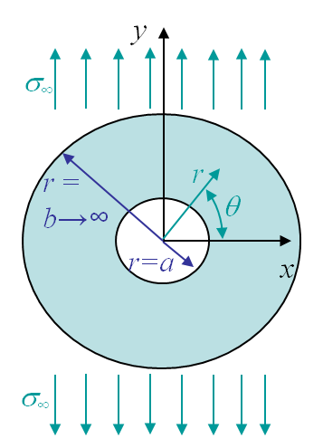
The problem of an infinite plate with a hole illustrated in Picture II.2 can be treated in cylindrical coordinates as shown in Picture II.5. Remember how to express the gradient operator in polar coordinates:
\begin{equation} \left( \begin{array}{c} \partial_{x} \\ \partial_{y} \end{array}\right) =\left(\begin{array}{cc} \cos{\theta} & -\frac{\sin{\theta}}{r}\\ \sin{\theta} & \frac{\cos{\theta}}{r} \end{array}\right) \left(\begin{array}{c} \partial_r\\ \partial_\theta
\end{array}\right) .\label{eq:rotGrad}\end{equation}
Using this last result, the Laplacian $\nabla^2$ operator is straightforwardly obtained as $ \left(\partial^2_{rr}+\frac{1}{r}\partial_r \frac{1}{r^2}\partial^2_{\theta\theta}\right)$, and the bi-harmonic equation (\ref{eq:biharmonic}) becomes
\begin{align} &\nabla^2 \nabla^2 \Phi = 0 \iff\nonumber\\ &\left(\partial^2_{rr}+\frac{1}{r}\partial_r \frac{1}{r^2}\partial^2_{\theta\theta}\right)\left(\Phi_{,rr}+\frac{1}{r}\Phi_{,r} +\frac{1}{r^2}\Phi_{,\theta\theta}\right)=0 \label{eq:biharmonicPolar}.\end{align}
We have now to express the stress components in the polar coordinates in terms of the Airy function, or more exactly in terms of $\Phi_{,r}$, $\Phi_{,r\theta}$ ... To change a tensor, as the stress tensor, from Cartesian to polar coordinates, one needs to apply
\begin{equation} \left( \begin{array}{cc} \mathbf{\sigma}_{rr} & \mathbf{\sigma}_{r\theta}\\ \mathbf{\sigma}_{r\theta} & \mathbf{\sigma}_{\theta \theta} \end{array}\right) =\left(\begin{array}{cc} \cos{\theta} & \sin{\theta}\\ -\sin{\theta} & \cos{\theta}
\end{array}\right) \left(\begin{array}{cc} \mathbf{\sigma}_{xx} & \mathbf{\sigma}_{xy}\\ \mathbf{\sigma}_{xy} & \mathbf{\sigma}_{yy}
\end{array}\right) \left(\begin{array}{cc} \cos{\theta} & \sin{\theta}\\ -\sin{\theta} & \cos{\theta} \end{array}\right)^T, \label{eq:rotTens} \end{equation}
which leads to
\begin{equation}\begin{cases} \mathbf{\sigma}_{rr} = & \mathbf{\sigma}_{xx} \cos^2{\theta} + \mathbf{\sigma}_{yy} \sin^2{\theta} + 2 \mathbf{\sigma}_{xy} \sin{\theta}\cos{\theta} \\ \mathbf{\sigma}_{\theta\theta} = & \mathbf{\sigma}_{yy} \cos^2{\theta} + \mathbf{\sigma}_{xx} \sin^2{\theta} - 2 \mathbf{\sigma}_{xy} \sin{\theta}\cos{\theta} \\ \mathbf{\sigma}_{r\theta} = & \left(\mathbf{\sigma}_{yy} - \mathbf{\sigma}_{xx}\right) \sin{\theta}\cos{\theta} + \mathbf{\sigma}_{xy}\left(\cos^2{\theta} - \sin^2{\theta}\right)\end{cases}. \label{eq:stressPolar} \end{equation}
The stress components in the Cartesian coordinates are known from (\ref{eq:Airy}) and read
\begin{equation}\begin{cases} \mathbf{\sigma}_{xx} = & \Phi_{,yy} \\ \mathbf{\sigma}_{yy} = & \Phi_{,xx} \\ \mathbf{\sigma}_{xy} = & -\Phi_{,xy}\end{cases} \label{eq:Airy2}. \end{equation}
Eventually, substituting (\ref{eq:Airy2}) in (\ref{eq:stressPolar}) leads to the expression of the stress components in terms of the Airy function, everything being stated in polar coordinates,
\begin{equation}\begin{cases} \mathbf{\sigma}_{rr} = & \frac{1}{r}\Phi_{,r}+\frac{1}{r^2}\Phi_{,\theta\theta} \\ \mathbf{\sigma}_{\theta\theta} = & \Phi_{,rr} \\ \mathbf{\sigma}_{r\theta} = & -\frac{1}{r}\Phi_{,r\theta}+\frac{1}{r^2}\Phi_{,\theta} \label{eq:AiryPolar} \end{cases}.\end{equation}
The problem is thus stated as finding $\Phi$ so that (\ref{eq:biharmonicPolar}) is satisfied as well as the boundary conditions. For the problem illustrated in Picture II.5, these boundary conditions (BCs) expressed in polar coordinates read:
-
At $r=a$, we have a stress free boundary:
\begin{equation} \mathbf{\sigma}_{rr}\left(r=a,\theta\right) = \mathbf{\sigma}_{r\theta}\left(r=a,\theta\right) = 0. \label{eq:plateHoleBc1} \end{equation} -
At $r =b \rightarrow \infty$, far away from the hole we should recover the uniform stress field $\sigma_{yy} = \sigma_\infty$:
\begin{equation} \begin{cases}\mathbf{\sigma}_{rr}\left(r=b,\theta\right) = \sigma_\infty \sin^2{\theta} = \frac{1}{2}\sigma_\infty - \frac{1}{2}\sigma_\infty \cos{2\theta}\\ \mathbf{\sigma}_{r\theta}\left(r=b,\theta\right) =\sigma_\infty \cos{\theta}\sin{\theta} = \frac{1}{2}\sigma_\infty \sin{2\theta}\end{cases}, \label{eq:plateHoleBc2} \end{equation}
where we have used (\ref{eq:stressPolar}). For this BC, one term is independent from the angle $\theta$, while the other terms depend on $2\theta$. This motivates to consider two different problems with two different BCs.
Load case 1: BCs independent from the angle
Let us consider the part of the BCs (\ref{eq:plateHoleBc1}-\ref{eq:plateHoleBc2}) independent from the angle
\begin{equation}\begin{cases} \mathbf{\sigma}_{rr}\left(r=a,\theta\right) = & \mathbf{\sigma}_{r\theta}\left(r=a,\theta\right) = 0 \\ \mathbf{\sigma}_{rr}\left(r=b,\theta\right) = & \frac{1}{2}\sigma_\infty \end{cases}.\label{eq:plateHoleBCLoad1}\end{equation}
The direct consequence is that the solution should also be independent from $\theta$ and can thus be written $\Phi\left(r\right)$. The bi-harmonic equation (\ref{eq:biharmonicPolar}) simplifies into
\begin{equation} \left(\partial^2_{rr}+\frac{1}{r}\partial_r\right)\left(\Phi_{,rr}+\frac{1}{r}\Phi_{,r}\right)=0, \end{equation}
which admits the general solution
\begin{equation} \Phi = C_1 \ln{r} + C_2 r^2 \ln{r} + C_3 r^2 + C_4 \label{eq:genSolLoad1}. \end{equation}
The four constants $C_1$, $C_2$, $C_3$ and $C_4$ are obtained by substituting (\ref{eq:genSolLoad1}) into (\ref{eq:AiryPolar})
\begin{equation}\begin{cases} \mathbf{\sigma}_{rr} = & \frac{1}{r}\Phi_{,r} = \frac{C_1}{r^2} +C_2\left(1+2\ln{r}\right) + 2 C_3 \\ \mathbf{\sigma}_{\theta\theta} = & \Phi_{,rr} = -\frac{C_1}{r^2} +C_2\left(3+2\ln{r}\right) + 2 C_3 \\ \mathbf{\sigma}_{r\theta} = & 0 \label{eq:stress1Load1} \end{cases},\end{equation}
which should satisfy (\ref{eq:plateHoleBCLoad1}). On the internal boundary, this means
\begin{equation} \frac{C_1}{a^2} +C_2\left(1+2\ln{a}\right) + 2 C_3 = 0, \end{equation}
and on the external boundary, this means
\begin{equation} \lim_{b\rightarrow \infty} \left(\frac{C_1}{b^2} +C_2\left(1+2\ln{b}\right) + 2 C_3\right) = \frac{1}{2}\sigma_\infty.\end{equation}
The constants can thus be directly computed as
\begin{equation}\begin{cases} C_1= & -\frac{a^2}{2}\sigma_\infty \\ C_2= & 0 \\ C_3= & \frac{1}{4}\sigma_\infty \end{cases},\end{equation}
and the stress components (\ref{eq:stress1Load1}) become
\begin{equation}\begin{cases} \mathbf{\sigma}_{rr} = & \frac{1}{2}\sigma_\infty\left(1- \frac{a^2}{r^2}\right) \\ \mathbf{\sigma}_{\theta\theta} = & \frac{1}{2}\sigma_\infty\left(\frac{a^2}{r^2}+1\right) \\ \mathbf{\sigma}_{r\theta} = 0\end{cases}.\label{eq:stressLoad1} \end{equation}
Load case 2: BCs dependent on the angle
Let us now consider the part of the BCs (\ref{eq:plateHoleBc1}-\ref{eq:plateHoleBc2}) dependent on the angle:
\begin{equation}\begin{cases} \mathbf{\sigma}_{rr}\left(r=a,\theta\right) = & \mathbf{\sigma}_{r\theta}\left(r=a,\theta\right) = 0 \\ \mathbf{\sigma}_{rr}\left(r=b,\theta\right) = & - \frac{1}{2}\sigma_\infty \cos{2\theta} \\ \mathbf{\sigma}_{r\theta}\left(r=b,\theta\right) = & \frac{1}{2}\sigma_\infty \sin{2\theta} \end{cases}.\label{eq:plateHoleBCLoad2}\end{equation}
In this case, the Airy function should have a dependency in $2\theta$. Let us assume that the solution has the shape
\begin{equation} \Phi=g\left(r\right)\cos{\left(2\theta\right)}.\label{eq:PhitmpBCLoad2}\end{equation}
The bi-harmonic equation (\ref{eq:biharmonicPolar}) thus becomes
\begin{equation}\begin{cases} \left(\partial^2_{rr}+\frac{1}{r}\partial_r +\frac{1}{r^2}\partial^2_{\theta\theta}\right)\left[\left(g''+\frac{g'}{r}-\frac{4g}{r^2}\right)\cos{2\theta}\right]=0 \\ \iff \left(g''''+ \frac{2g'''}{r} - \frac{9g''}{r^2}+\frac{9g'}{r^3}\right)\cos{2\theta}=0\end{cases}, \end{equation}
which is satisfied by the general solution
\begin{equation} \Phi = \underbrace{\left(C_1 r^4 +C_2r^2+\frac{C_3}{r^2}+C_4\right)}_{g\left(r\right)}\cos{2\theta} . \label{eq:PhiBCLoad2} \end{equation}
Replacing this expression into (\ref{eq:AiryPolar}) leads to the components of the stress tensor
\begin{equation}\begin{cases} \mathbf{\sigma}_{rr} = & \left(\frac{g'}{r}-\frac{4g}{r^2}\right)\cos{2\theta}=\left(-2C_2-\frac{6C_3}{r^4}-\frac{4C_4}{r^2}\right)\cos{2\theta} \\ \mathbf{\sigma}_{\theta\theta} = & g''\cos{2\theta}=\left(12C_1r^2+2C_2+\frac{6C_3}{r^4}\right)\cos{2\theta} \\ \mathbf{\sigma}_{r\theta} = & \left(\frac{2g'}{r}-\frac{2g}{r^2}\right)\sin{2\theta}=\left(6C_1r^2+2C_2-\frac{6C_3}{r^4}-\frac{2C_4}{r^2}\right)\sin{2\theta} \end{cases},\label{eq:stress1Load2}\end{equation}
which should satisfy (\ref{eq:plateHoleBCLoad2}), yielding the following values for the constants:
\begin{equation}\begin{cases} C_1 = & 0 \\ C_2 = & \frac{\sigma_\infty}{4} \\ C_3 = & \frac{\sigma_\infty a^4}{4} \\ C_4 = & -\frac{\sigma_\infty a^2}{2} \end{cases}.\end{equation}
Finally, when replacing the constants in (\ref{eq:stress1Load2}), the components of the stress tensor now read
\begin{equation}\begin{cases} \mathbf{\sigma}_{rr} = & \frac{\sigma_\infty}{2}\left(\frac{4a^2}{r^2}-1-\frac{3a^4}{r^4}\right)\cos{2\theta} \\ \mathbf{\sigma}_{\theta\theta} = & \frac{\sigma_\infty}{2} \left(1+\frac{3a^4}{r^4}\right)\cos{2\theta} \\ \mathbf{\sigma}_{r\theta} = & \frac{\sigma_\infty}{2} \left(1-\frac{3a^4}{r^4}+\frac{2a^2}{r^2}\right)\sin{2\theta} \end{cases}\label{eq:stressLoad2}.\end{equation}
Superposition of load cases 1 and 2
The stress field of the initial problem is obtained by adding the stress components (\ref{eq:stressLoad1}) and (\ref{eq:stressLoad2}) of the two load cases, leading to
\begin{equation}\begin{cases} \mathbf{\sigma}_{rr} = & \frac{\sigma_\infty}{2}\left[\left(\frac{4a^2}{r^2}
-1-\frac{3a^4}{r^4}\right)\cos{2\theta} + 1- \frac{a^2}{r^2}\right] \\ \mathbf{\sigma}_{\theta\theta} = & \frac{\sigma_\infty}{2} \left[\left(1
+\frac{3a^4}{r^4}\right)\cos{2\theta}
+ \frac{a^2}{r^2}+1\right] \\ \mathbf{\sigma}_{r\theta} = & \frac{\sigma_\infty}{2}
\left(1-\frac{3a^4}{r^4}+\frac{2a^2}{r^2}\right)\sin{2\theta} \end{cases}\label{eq:stressHole}.\end{equation}
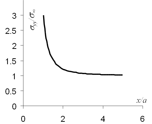
The stress evolution of interest for the problem of an infinite plate with a hole is $\mathbf{\sigma}_{yy}\left(x,\,y=0\right)$, which corresponds to $\mathbf{\sigma}_{\theta\theta}\left(r,\,\theta=0\right)$, and which is obtained from (\ref{eq:stressHole})
\begin{equation}
\mathbf{\sigma}_{yy}\left(x,y=0\right) = \frac{\sigma_\infty}{2} \left(2
+\frac{3a^4}{x^4}+ \frac{a^2}{x^2}\right)
\end{equation}
The evolution of this stress field is illustrated on Picture II.6. When the ratio between $r$ and $x$ tends to 1, meaning at the hole boundary, the stress concentration factor (which is not a stress intensity factor) for a circle tends to $K_\text{circle}=3$.
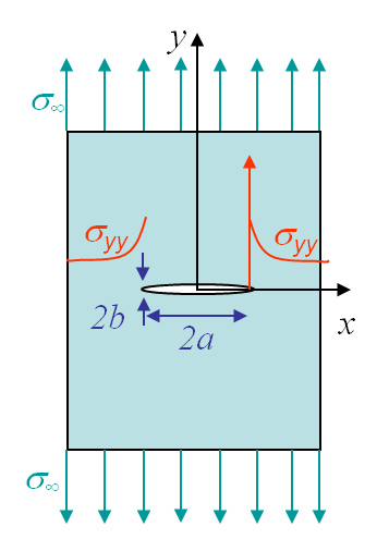
Application: infinite plate with an elliptical hole
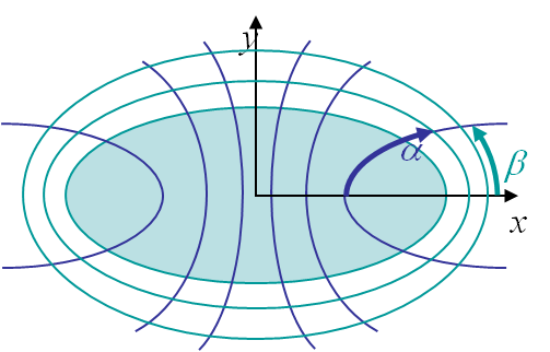
The problem of an infinite plate with an elliptical hole, shown in Picture II.3, can be solved by considering the elliptical coordinates illustrated on Picture II.7, which read
\begin{equation}\begin{cases} x = & c \cosh{\alpha}\cos{\beta}\\ y = & c \sinh{\alpha}\sin{\beta} \end{cases}.\end{equation}
The inner hole of large and small radii $a$ and $b$ is thus represented by $\alpha=\alpha_0$ and the parameter $c$ as
\begin{equation}\begin{cases} c \cosh{\alpha_0}= & a \\ c \sinh{\alpha_0}= & b \end{cases}.\end{equation}
The problem can be solved by considering a complex function $z = c \cosh{\zeta}$ of the complex variable $\zeta = \alpha+i\beta$. Doing so Inglis (1913) has computed the maximum stress as
\begin{equation} \sigma_\text{max} = \sigma_{yy} (a,0) = \sigma_\infty \left( 1+\frac{2a}{b} \right), \end{equation}
leading to a stress concentration factor $K_\text{ell} = 1+\frac{2a}{b} = 1+2\sqrt{\frac{a}{\rho}}$ where $\rho$ is the curvature radius of the hole at $x=a$. We observe a singularity when $\rho \rightarrow 0$.
![]()