
\(\newcommand{\cauchy}{\boldsymbol{\sigma}}\) \(\newcommand{\strain}{\boldsymbol{\varepsilon}}\) \(\newcommand{\uV}{\boldsymbol}\) \(\newcommand{\uT}{\boldsymbol}\) \(\newcommand{\defu}{\boldsymbol{u}}\)
J-integral > $J$-controlled crack growth
Resistance curve & crack stability
In the lecture on crack growth, we have introduced the concept of resistance curve. As a reminder, the active plastic zone moves with the crack tip in case of crack growth, meaning that the crack is opening in a zone affected by permanent plastic deformations: the plastic wake. This makes the crack more difficult to be opened, which corresponds to an increase of the apparent fracture energy $G_C$ with the crack propagation $\Delta a$. This defines the resistance curve $J_R(a)$, and its evaluation in the case of ductile materials has been detailed in the previous section in terms of the evolution of the $J$-integral during a toughness test.
It is thus possible to assess a crack stability, in the same way as it has been done in LEFM, by comparing the evolution of $J(a)$ with the resistance curve $R_c(a)$ in terms of their derivatives: $\partial_a J(a) <?>\partial_a J_R(a)$. However, as it was lengthy discussed, the theory behind the $J$-integral assumes a proportional loading, which is not the case when a crack propagates since this involves partial unloading. Therefore the question which remains is "Under which condition can the $J$-integral be evaluated during a crack propagation?"
$J$-controlled region
Definition
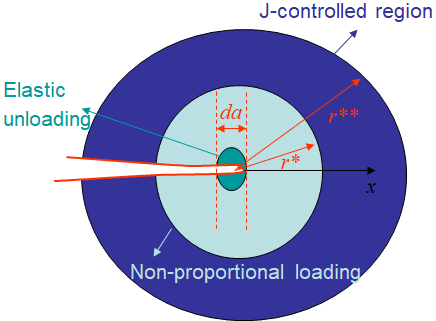
Let us assume that the crack propagates on a distance $da$ as illustrated in Picture IX.29. Clearly, since the crack lips are stress-free, there is a "green region" in the vicinity of the crack increment, which scales with $da$, in which the material is elastically unloaded. As a consequence there exists a "light blue" zone of radius $r^*$ in which the loading is non-proportional during the crack propagation. Besides, remembering that the HRR solution is an asymptotic one, the stress and strain fields are governed by the $J$-integral in a bounded zone of radius $r^{**}$ from the crack tip.
Therefore, for the $J$-integral to be meaningful during a crack propagation, there is a requirement that there still exists a "dark blue" annular region separated by the radii $r^*$ and $r^{**}$ in which the stress and strain fields are governed by the $J$-integral, this is the $J$-controlled region.
Existence
One obvious condition for the $J$-controlled region to exist is that the crack increment remains limited in comparison with the zone in which the HRR theory is valid:
\begin{equation} da<<r^{**} .\label{eq:JcontrolledCond1}\end{equation}
The other condition is assessed by evaluating the size of the zone of non-proportional loading of radius $r^*$. Assuming it exists, in the zone of $J$-controlled region, the strain follows
\begin{equation}\label{eq:strain_Jintbis} \strain=\frac{\sigma_p^0\alpha}{E}\left(\frac{J E}{r\alpha\left(\sigma_p^0\right)^2I_n}\right)^{\frac{n}{n+1}} \tilde{\strain}\left(\theta,\,n\right). \end{equation}
Since the strain field depends on both the crack length and the $J$-integral, one has
\begin{equation}d\strain = \partial_a \strain da + \partial_J \strain dJ,\label{eq:dstrain} \end{equation}
The second term of the right hand side of Eq. (\ref{eq:dstrain}) is directly obtained from Eq. (\ref{eq:strain_Jintbis}), with
\begin{equation} \partial_J \strain = \frac{n}{n+1}\frac{\sigma_p^0\alpha}{E} \left(\frac{JE}{r\alpha\left(\sigma_p^0\right)^2I_n}\right)^{\frac{n}{n+1}}\frac{1}{J} \tilde{\strain}\left(\theta,\,n\right).\label{eq:dstraindJ} \end{equation}
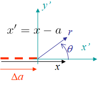
To evaluate the first term of the right hand side of Eq. (\ref{eq:dstrain}), we consider a polar referential linked to the crack tip as illustrated in Picture IX.30, with $x'=x-a$. Therefore, the derivative with respect to the crack advance reads
\begin{equation} \partial_a = -\partial_{x'} = - \cos{\theta}\partial_r +\frac{\sin{\theta}}{r}\partial_\theta. \label{eq:chgevar} \end{equation}
We thus need to evaluate the derivative of the strain field (\ref{eq:strain_Jintbis}) with respect to the distance $r$, with
\begin{equation} \partial_r \strain = - \frac{n}{n+1}\frac{\sigma_p^0\alpha}{E} \left(\frac{JE}{r\alpha\left(\sigma_p^0\right)^2I_n}\right)^{\frac{n}{n+1}}\frac{1}{r} \tilde{\strain}\left(\theta,\,n\right),\label{eq:dstraindr} \end{equation}
and with respect to the direction $\theta$, with
\begin{equation} \partial_\theta \strain = \frac{\sigma_p^0\alpha}{E} \left(\frac{JE}{r\alpha\left(\sigma_p^0\right)^2I_n}\right)^{\frac{n}{n+1}} \partial_\theta\tilde{\strain}\left(\theta,\,n\right). \label{eq:dstraindtheta}\end{equation}
Therefore, defining
\begin{equation} \tilde{\tilde{\strain}}\left(\theta,\,n\right) = \frac{n}{n+1} \cos{\theta}\tilde{\strain}+\sin{\theta}\partial_\theta\tilde{\strain} ,\label{eq:tildetildestrain} \end{equation}
the combination of Eqs. (\ref{eq:chgevar}-\ref{eq:dstraindr}) leads to
\begin{equation} \partial_a \strain = \frac{\sigma_p^0\alpha}{E} \left(\frac{JE}{r\alpha\left(\sigma_p^0\right)^2I_n}\right)^{\frac{n}{n+1}}\frac{1}{r} \tilde{\tilde{\strain}}\left(\theta,\,n\right) .\label{eq:dstrainda}\end{equation}
Eventually, using Eqs. (\ref{eq:dstraindJ}) and (\ref{eq:dstrainda}), the relation (\ref{eq:dstrain}) becomes
\begin{equation} d \strain = \frac{\sigma_p^0\alpha}{E} \left(\frac{JE}{r\alpha\left(\sigma_p^0\right)^2I_n}\right)^{\frac{n}{n+1}}\left(\frac{n}{n+1}\frac{dJ}{J} \tilde{\strain} +\frac{da}{r} \tilde{\tilde{\strain}}\right). \label{eq:dstrainfinal}\end{equation}
Since both $\tilde{\strain}$ and $\tilde{\tilde{\strain}}$ are independent on $r$ and are on the same order of magnitude, and since only the term $\frac{da}{r}$ includes a non-proportional loading (since in $\frac{1}{r}$), the existence of the $J$-controlled region implies that this latter term can be neglected, i.e. that
\begin{equation} \frac{dJ}{J} >> \frac{da}{r}, \label{eq:existenceJzonetmp}\end{equation}
or again
\begin{equation} r >> \frac{J}{\frac{dJ}{da}}. \label{eq:existenceJzone}\end{equation}
During a fracture toughness test, the resistance curve $J_R(\Delta a)$ can be extracted allowing to evaluate at crack initiation the following material characteristic dimension
\begin{equation} D = J_{IC}/\left.\frac{dJ}{d\Delta a}\right|_c. \label{eq:Dtoughness} \end{equation}
As a result, the second condition, besides Eq. (\ref{eq:JcontrolledCond1}), for a $J$-controlled zone to exist reads
\begin{equation} D << r^{**}.\label{eq:JcontrolledCond2} \end{equation}
In practice, the length $r^{**}$ is test-dependent and can be obtained by using the finite-element method. Typically it is expressed as a fraction of the ligament $L-a$ or of another characteristic length such as the plastic zone $r_p$.
Crack stability and tearing
Assuming both conditions (\ref{eq:JcontrolledCond1}) and (\ref{eq:JcontrolledCond2}) are satisfied, there exists a $J$-controlled zone during crack propagation, and the crack stability is assessed by comparing the growth of the $J$-integral, which is geometry and loading-dependent, with the slope of the material resistance curve, i.e.
\begin{equation} \frac{dJ\left(a,\,Q\right)}{da} <\left.\frac{dJ_R}{d a}\right|_{\Delta a=0} .\label{eq:JstabilityTmp}\end{equation}
In order to use non-dimensional entities, one can define the, geometry and loading-dependent, tearing as
\begin{equation} T =\frac{E}{\left(\sigma_p^0\right)^2} \frac{dJ\left(a,\,Q\right)}{da}\,, \label{eq:tearing}\end{equation}
and the critical tearing, which is a material value, but might depend on the test specimen considered for its evaluation,
\begin{equation} T_0 =\frac{E}{\left(\sigma_p^0\right)^2} \left.\frac{dJ_R}{da}\right|_{\Delta a=0}\,.\label{eq:tearing0}\end{equation}
The crack stability condition (\ref{eq:JstabilityTmp}) thus becomes
\begin{equation} T < T_0 .\label{eq:Jstability}\end{equation}
Typical values obtained for toughness tests on a Compact Tension specimen are reported here below for indication purpose only. In particular, one wants to observe the difference of values between ductile materials such as steel, and the more brittle aluminum alloy. Note also the effect of the temperature, which is not monotonic.
| Material | Specimen | Temperature [$\deg$ C] | $\frac{\sigma_p^0+\sigma_{\text{TS}}}{2}$ [MPA] | $J_{IC}$ [MPA$\cdot$m] | $\frac{dJ}{da}$ [MPA] | $T$ [-] | $D $ [mm] |
|---|---|---|---|---|---|---|---|
ASTM 470 (Cr-Mo-V) |
CT | 149 |
621 |
0.084 |
48.5 |
25.5 |
1.78 |
260 |
621 |
0.074 |
49 |
25.8 |
1.52 |
||
427 |
592 |
0.088 |
84 |
48.6 |
1.01 |
||
ASTM A453 (Stainless steel) |
CT | 24 |
931 |
0.124 |
141 |
32.8 |
|
204 |
820 |
0.107 |
84 |
25.6 |
1.27 |
||
427 |
772 |
0.092 |
65 |
22.4 |
|||
6061-T651 (Aluminum) |
CT | 24 |
298.2 |
0.0178 |
3.45 |
2.79 |
5 |