
\(\newcommand{\cauchy}{\boldsymbol{\sigma}}\) \(\newcommand{\strain}{\boldsymbol{\varepsilon}}\) \(\newcommand{\uV}{\boldsymbol}\) \(\newcommand{\uT}{\boldsymbol}\) \(\newcommand{\defu}{\boldsymbol{u}}\)
J-integral > Fracture toughness testing for elasto-plastic materials
In the previous section, we have seen how to evaluate the $J$-integral of a cracked body. In this section we will apply these methods to assess the maximum $J$-integral that an elasto-plastic material can sustain.
Normalized procedure
The purpose of fracture toughness testing in the case of elasto-plastic materials is to evaluate limit values of the $J$-integral in order to further assess the behavior of a cracked body. In particular we are interested in three values
- The plane-$\varepsilon$ value of $J$ prior to significant crack growth: $J_C$;
- The plane-$\varepsilon$ value of $J$ near the onset of stable crack growth: $J_{IC}$;
- The evolution of $J$ with the crack growth $\Delta a$ as a resistance curve for stable crack growth: $J_R(\Delta a)$.
Plane-$\varepsilon$ conditions are usually considered for conservatism reasons as it will be justified later.
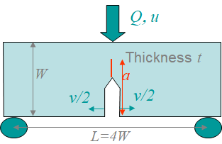
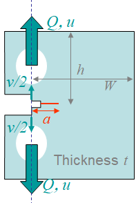
The testing process should strictly follow the norm, e.g. the ASTM E1820 norm, and is usually performed on either the Single Edge Notch Bend (SENB) specimen, see Picture IX.22, or on the Compact Tension Specimen (CTS), see Picture IX.23. During the sample loading, the evolution of the crack mouth opening $v$ is measured since it is more accurate than the measurement of the deflection $u$. The testing process will be summarized in the following section.
R-curve method
First step: Fatigue crack growth
A cracked sample cannot be manufactured in representative way. Therefore, the samples are manufactured with a notch, and a crack is initaited and grown by fatigue. To this end a cyclic loading reaching the maximum load $Q_\text{fat}$ is applied to the notched sample. In order to avoid plastic flow during the unloading stage, the last three cycles are in between $\frac{Q_\text{fat}}{2}$ and $Q_\text{fat}$.
Before conducting the toughness test, one needs to know what the initial size $a_0$ of the crack originating from the fatigue loading is. An accurate measurement is not possible, so we estimate the compliance of the sample and use formula that have been obtained by finite element analyzes of the normalized sample with different crack lengths $a$. Since we are not propagating the crack at this stage, the formula are the ones of linear elasticity, and imply to apply a reduced loading $Q$. As previously stated, the measurement of the crack mouth opening $v$ is more accurate than that of the deflection $u$, and the compliance is thus defined in terms of $\frac{v}{Q}$.
For the SENB specimen, the following relation of the crack length in terms of the normalized compliance $U$ has been derived:
\begin{equation}\begin{cases} \frac{a}{W} &= 0.9997-3.95 U +2.982 U^2-3.214 U^3 + 51.52 U^4 - 113.0 U^5;\text{ with}\\ U&= \frac{1}{1+\sqrt{\frac{4E't v W}{LQ}}}.\end{cases}\label{eq:SENBcrack} \end{equation}
These formula can be inverted in order to define the elastic compliance $C_e$ for a known crack length, leading to, for the SENB specimen
\begin{equation} C_e=\frac{v}{Q} = 6 \frac{L}{E'tW}\frac{a}{W}\left[0.76-2.28\frac{a}{W}+3.87\left(\frac{a}{W}\right)^2-2.04\left(\frac{a}{W}\right)^3+\frac{0.66}{\left(1.-\frac{a}{W}\right)^2}\right].\label{eq:SENBvCompliance} \end{equation}
We finally note that similar formula exist when considering the elastic compliance $C_{LLe}$ in terms of the deflection $u$, with for the SENB specimen
\begin{equation} C_{LLe}=\frac{u}{Q} = \frac{1}{E't}\left(\frac{L}{W-a}\right)^2 \left[1.193-1.98\frac{a}{W}+4.478\left(\frac{a}{W}\right)^2-4.443\left(\frac{a}{W}\right)^3+1.739\left(\frac{a}{W}\right)^4\right]. \label{eq:SENBuCompliance}\end{equation}
Second step: Sample loading
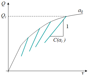
Once the initial crack length $a_0$ has been determined, the toughness test can proceed. To this end the load $Q$ is increased and the crack mouth opening $v$ recorded. Once the crack starts propagating, several cycles of partial unloading/reloading are applied, see Picture IX.24. During the loading, the crack size increases and the partial unloading steps are necessary to determine its evolution using the compliance method, e.g. using Eqs. (\ref{eq:SENBcrack}) for the SENB specimen. The unloading stages are partial, i.e. the load is not decreased down to zero in order to avoid reverse plasticity at crack tip.
Once enough, i.e. at least 8, pairs $(a_i,\,Q_i)$ of crack length and loading have been obtained, the sample is totally unloaded and broken (after cooling down if needed to reduce the required load), and the final crack is marked.
Third step: Data reduction
We can now evaluate the evolution of the $J$-integral during the crack propagation using the $\eta$-approach. To this end, for each pair $(a_i,\,Q_i)$, one has to
- Calculate the elastic part of the $J$-integral with \begin{equation} J_{e,\,i} = \frac{K_I^2\left(a_{i}\right)}{E'}.\label{eq:Jei}\end{equation} The stress intensity factor is determined using formula derived using LEFM and in particular using the finite element method. For the SENB specimen, the following expression is given by the norm: \begin{equation}
\begin{array}{ll}K_I=&\frac{QL}{tW^{\frac{3}{2}}}\\ &\frac{3\sqrt{\frac{a}{W}}\left[1.99-
\frac{a}{W}\left(1-\frac{a}{W}\right) \left(2.15-3.93\frac{a}{W}+2.7\left(\frac{a}{W}\right)^2\right)\right]} {2\left(1+2\frac{a}{W}\right)\left(1-\frac{a}{W}\right)^\frac{3}{2}}.\end{array}\label{eq:KISENB}\end{equation}
- Evaluate the plastic part of the deflection with \begin{equation} u_{p,\,i} = u_i - Q_i C_{LLe}\left(a_i\right),\label{eq:upi} \end{equation} where the elastic compliance $C_{LLe}$ in terms of the deflection $u$ is also obtained under the form of derived formula, e.g. Eq. (\ref{eq:SENBuCompliance}) for the SENB specimen.
- Evaluate the increment in the plastic work during a crack increment $a_i-a_{i-1}$ as \begin{equation}\Delta W^p_i = \int_{u_{p,\,i-1}}^{u_{p,\,i}} Q du_p' .\label{eq:Wpi} \end{equation}
- Evaluate the plastic part of the $J$-integral using the $\eta$-approach, yielding \begin{equation} J_{p,\,i}=J_{p,\,i-1}+\frac{\eta_p}{t}\Delta W^p_i \frac{W-a_i}{\left(W-a_{i-1}\right)^2}\label{eq:Jpincrement}, \end{equation} with $\eta_p=2$ for the SENB specimen. Note that the term $\frac{W-a_i}{\left(W-a_{i-1}\right)^2}$ is used as an approximation of the average ligament size during the crack increment $a_i-a_{i-1}$.
- Evaluate the final $J$-integral with \begin{equation}J_i=J_{e,\,i} + J_{p,\,i}.\label{eq:Ji} \end{equation}
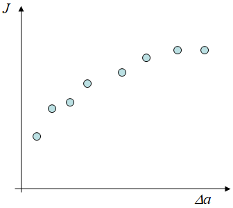
Using these values $J_i$ evaluated for the different crack lengths $a_i$ allows drawing the $J$-$\Delta a$ curve, see Picture IX.25, with $\Delta a=a-a_0$ computed from the initial crack length $a_0$.
Fourth step: Analysis
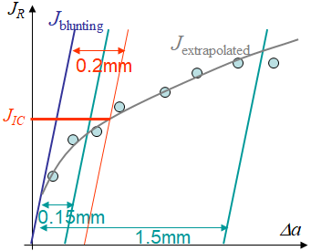
We can now analyze the data $(J_i,\,a_i)$ of Picture IX.25 following the approach illustrated in Picture IX.26 in order to determine the values of interest. To do so, we proceed as follows
- First, even before the crack starts to growth, there is a blunting of the crack tip, which corresponds to an apparent $\Delta a$. Indeed, remembering the evaluation of the crack tip opening displacement, it appears that the crack tip opening displacement $\delta_t$ is measured at a distance $r^*$ with $ r^*-\defu_x\left(r^*,\,\pi\right) = \defu_y\left(r^*,\,\pi\right)=\frac{\delta_t}{2}$. However, since $J=\frac{\sigma_p^0\delta_t}{d_n}$, we can approximate the apparent $J$ resulting from the crack tip opening as \begin{equation} J_\text{blunting} = 2\sigma_p^0 \Delta a;\label{eq:bluntingThoughness} \end{equation} This so-called blunting line is reported in Picture IX.26.
- Second, two exclusion lines are drawn parallel to the blunting line and shifted by values of $\Delta a$ equal to $0.15\text{mm}$ and $1.5\text {mm}$. The $J$-line evolution is then extrapolated using the points between these two exclusion lines following \begin{equation} \ln J =\ln C_1+ C_2\ln \Delta a. \label{eq:lnJToughness}\end{equation}
- Third, the plane-$\varepsilon$ value of $J$ near the onset of stable crack growth, $J_{IC}$, is defined as the intersection of the extrapolated $J$-line (\ref{eq:lnJToughness}) and the $0.2\text{ mm}$ line offset from the blunting line, see Picture IX.26.. Validity of the analysis is now checked by comparing $J_{IC}$ to the crack tip opening displacement, with in the case of the norm \begin{equation} t,\,W-a > 25\frac{J_{IC}}{\frac{\sigma_p^0+\sigma_{TS}}{2}}.\label{eq:checkToughness} \end{equation} If this equation is not satisfied, new thicker samples have to be manufactured.
- Fourth, if Eq. (\ref{eq:checkToughness}) is satisfied, the plane-$\varepsilon$ value of $J$ prior to significant crack growth, $J_C$, is defined as the intersection of the extrapolated $J$-line (\ref{eq:lnJToughness}) and the blunting line, see Picture IX.26.
- Fifth, the resistance curve for stable crack growth, $J_R(\Delta a)$, is defined as the evolution of the extrapolated $J$-line (\ref{eq:lnJToughness}) with the crack growth $\Delta a$ beyond $J_{IC}$.
Typical resistance curves
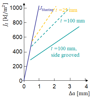
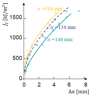
Picture IX.27 and Picture IX.28 illustrate typical resistance curves of a ductile material as can be found in "Andrews WR and Shih CF (1979), Thickness and side -groove effects on J- and d- resistance curves for A533-B steel at 93$^o$C, ASTM STP 668 , 426-450" for steel A533-B, values for indication purpose only. Picture IX.27 shows that the resistance curves, but also the values of $J_{IC}$, are not unique for a given material, but depend on the thickness of the sample. Actually, when the thickness increases, the stress-triaxiality tends to that of a plane-$\varepsilon$ state and the sample is less resistant to crack propagation. This behavior has been discussed in the HRR theory finding. This means that in order to ensure conservatism, the sample should be thick enough, justifying the condition (\ref{eq:checkToughness}). Another solution is to groove, i.e. dig half-cylindrical shapes in the alignment of the crack, both sides of the sample. In that way the plane-$\sigma$ state of the sample sides is cancelled, lowering the resistance curves. The values also depend, because of the change of triaxiality, on the other geometrical parameters such as the initial crack length in Picture IX.28, but to a lower extent.
![]()