
Overview
This chapter should be seen as a brief introduction to the different lessons. The different concepts introduced here will be explained in more details in the following chapters.
Overview > Fatigue
Historical background
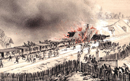
In the middle of the 19th century with the generalisation of the use of steam engines, especially for trains, engineers had to face a new kind of problem never really encountered before: some trains were suffering of severe damage, although the loading remains in the design range. One of the most famous accidents, the Versailles rail accident illustrated in Picture I.1, is due to the rail axle failure of the leading locomotive. However at that time the failure could not be explained.
One of the first engineers to investigate this issue was the German August Wöhler around 1860. His analysis led to the following conclusions:
- Failure did not occur at the first time the train was put into service, but after various times.
- Failure occurred at loads much lower than expected.
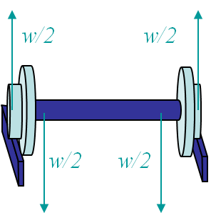
His conclusion was that the incidents were due to the fact that a train axle is submitted to a cyclic loading/unloading. Indeed an axle is submitted to a shear load due the weight of the train car, which in turns induces a bending moment in the axle, see Picture I.2. As the axle is rotating, a point of the axle isl alternatively submitted to compression and to traction when lying above or below the neutral axis, see Picture I.3. Due to this cyclic loading, the axle experiences fatigue and the life of the structure is limited. Based on this observation Wöhler has developed a theory based on an empirical approach: the total life theory.
Total life theory
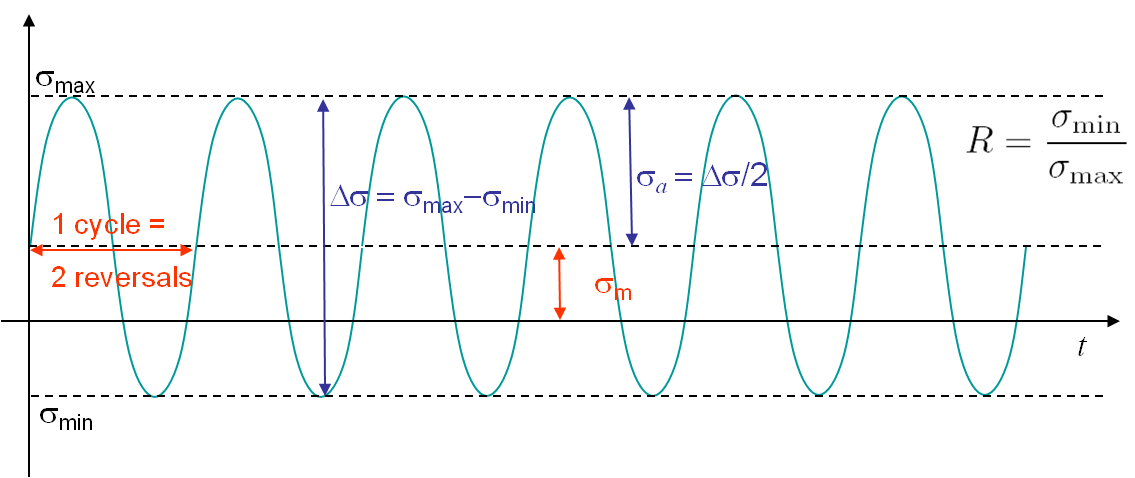
Based on experiments Wöhler found that the life of a structure submitted to a cyclic loading depends on two values characterizing this loading, see Picture I.3:
- The maximum stress reached during one cycle: $\sigma_\text{max}$ and
- The minimum stress reached during one cycle: $\sigma_\text{min}$.
Alternatively the cycle, and thus the life of the structure, is characterized by any two of the following values, see Picture I.3:
- The mean stress: $ \sigma_m = \frac{\sigma_\text{max} + \sigma_\text{min}}{2}, $
- The cycle amplitude: $ \sigma_a = \frac{1}{2}\Delta\sigma = \frac{1}{2} (\sigma_\text{max} - \sigma_\text{min})$, and
- The cycle loading ratio: $ R = \frac{\sigma_\text{min}}{\sigma_\text{max}}$.
Under particular environmental conditions such as high humidity, high temperature ... one also needs to consider the parameters related to the creep effect:
- The frequency $f_\text{cycle} = \frac{1}{T_\text{cycle}}$ of a cycle, where $T_\text{cycle}$ is the period of a cycle, and
- The shape of a cycle (sine, step, ...)
Once those values are known the limit cycles number (or life) in terms of the loading can be predicted using one of the two total life approaches summarized as:
Stress life approach
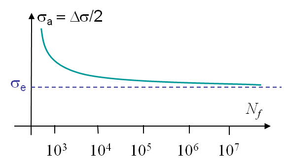
This approach can be used for structures experiencing essentially elastic deformations. By applying different cyclic loading on samples made of a given material, Wöhler has experimentally extracted curves predicting the limit cycles number $N_f$ (or life) in terms of the loading parameters: $\sigma_a = 0$ and $\sigma_m = 0$. An example of such a curve obtained for $\sigma_m = 0$ is illustrated in Picture I.4. It is important to note that a Wöhler curve is obtained
- For one material,
- For one cyclic condition (one value of $\sigma_m$), and
- Under the assumption of all the cycles being identical to each other.
For some materials there exists an endurance limit $\sigma_e$ defined as the stress state below which the structure can handle at least 107cycles. An order of magnitude for $\sigma_e$ is [0.35-0.5] of $\sigma_\text{TS}$ (tensile strength of the material), see Picture I.4.
Thus for a given structure, one generally knows the material while the loading ($\sigma_a$ and $\sigma_m$) can be computed at strain concentration zones, in which case the Wöhler curves directly give the limit cycles number $N_f$ of the structure.
One practial way of using the Wöhler curves is the recourse to the Basquin law (1910), which describes the curves for $\sigma_m=0$ as:
\begin{equation} \frac{\Delta \sigma}{2} = \sigma_a = \sigma'_f (2N_f)^b, \label{eq:basquin}\end{equation}
where
- $σ'_f$ is the fatigue coefficient -typical values at room temperature for mild steel are between 1 and 3 GPa,
- $b$ is the fatigue exponent -typical values at room temperature for mild steel are between -0.1 and -0.06.
Note that all these parameters are determined from experiments, which are time consuming as for a single material they require multiple tests, each of one implying millions of cycles.
Strain life approach
This approach is meant to be used for structures suffering locally plastic deformations. The Manson-Coffin law (1952) can be applied for identical cycles:
\begin{equation} \frac{\Delta \bar{\varepsilon}^p}{2} = \varepsilon'_f (2N_f)^c, \label{eq:mansonCoffin}\end{equation}
where
- $\Delta \bar{\varepsilon}^p$ is the plastic increment during the loading cycle,
- $\varepsilon'_f$ is the fatigue ductility coefficient -roughly equal to the true fracture ductility for metals, and
- $c$ is the fatigue ductility exponent -around -0.7 to -0.5 for metals.
Limits of the total life approach
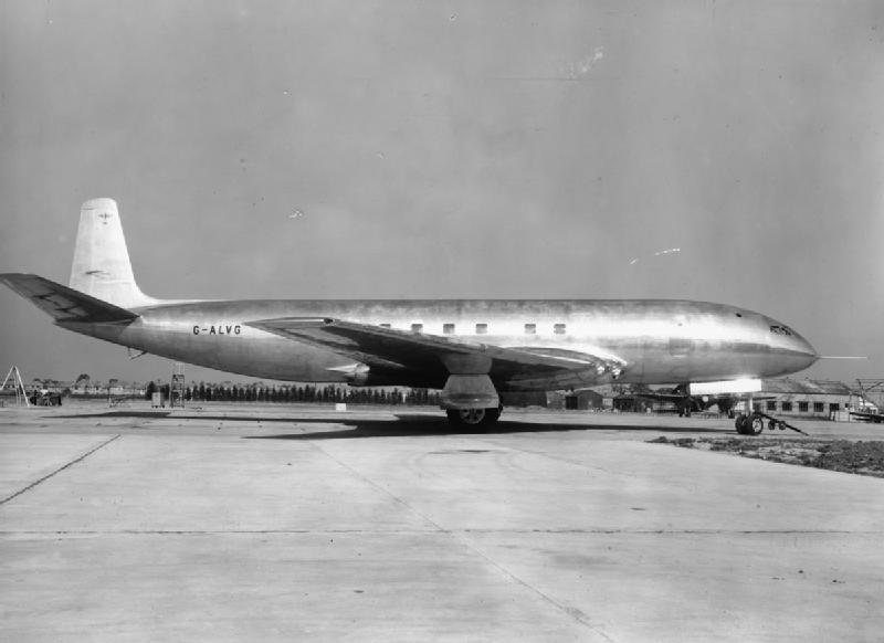
The total life approach is a purely empirical approach, which does not take into account the microscopic origin of fatigue. It has been successfully used for many years to design structures up to the middle of the 20th century, time at which its limits dramatically appeared with the arising of the first pressurized jetliner: the De Havilland 106 Comet 1 airplane whose first flight occured in 1952, see Picture I.5. This jetliner was able to transport 36 passengers in a pressurized cabin at 0.58 atm. Due to the pressurization, the fuselage experiences cyclic loading, and the airplane was designed for 10,000 cycles.
However, this plane suffered from design issues:
- A first one -not really related to this class- was purely on aerodynamics level and resulted in two planes failing to become airborne in 1952 and 1953. At high angles of attack, as during take-off, because of the swept wing a loss of lift could appear due to the span wise flow, which was solved by adding wing fences. Still at high angles of attack the air intake of the engines was insufficient.
- The jetliner family also experienced other fatal accidents, which first remained somehow unexplained. One of these accidents occurred in India in 1954 during a storm: the plane suffered from a structural failure at the stabilizer level. A first explanation was that the pilot, who had to achieve severe manoeuvers, overstressed the fully powered -through hydraulic assistance- stabilizer as he did not get a force feedback. Following this accident a feedback feel system was introduced so that the control column forces would be proportional to the control surface load.
- However, other accidents kept occurring. In January 1954, the plane registered G-ALYP flying from Rome to Heathrow (BOAC 781) fell in the sea after take-off. As the autopsies of the passenger's lung revealed an explosive decompression, either a bomb or a turbine failure was suspected to be responsible for the crash as fatigue was excluded: The plane had only 1,300 cycles while it was designed to last at least 10,000 cycles. So the turbine rings were armoured.
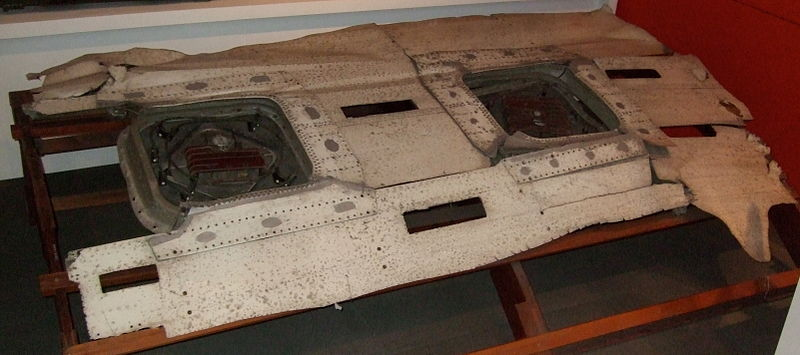
- In April 1954 another flight from Rome to Cairo disintegrated above the sea. Meanwhile the plane G-ALYP was reconstructed from the wreckages found in the sea, see Picture I.6. The investigators found out that the plane suffered from crack propagation in the fuselage, but the crack origin was still unknown.
- During the same month the engineers have performed a test which will finally allow the mode of failure to be discovered: they have simulated the pressurization cycles by filling in and pumping out the fuselage registered G-ALYU with water. The fuselage surprisingly failed after 3057 cycles at the port window due to a crack initiation and propagation, well below the design number of 10,000 cycles.
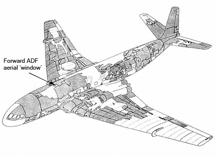
- In August 1954 the discovery of the roof of the G-ALYP confirmed this cause of failure. Indeed the engineers noticed that the crack has originated from the communication window corner, see Picture I.7.
Nevertheless, although the mode of the failure was identified, the origin was still unknown. Indeed the fuselage has been fatigue designed to sustain 10,000 cycles. Moreover a fuselage has been tested at the design stage and has sustained these 10,000 cycles. So how could one explain the in service failure for a much lower cycles number?
- The origin of failure lies in the microscopic defects which cannot be accounted for using the total life approach. Indeed, on the Comet 1, the windows were squared and riveted. The rivets were punched instead of being drilled to reduce the production cost, leading to the presence of micro-cracks. These initial defects being located at a high stress concentration area -because of the windows shape- were the sources for crack initiation and propagation. The total life approach would not account for the existence of micro-defects and failed to predict the real time life.
- But then how to explain that the tested fuselage at the design stage actually passed the fatigue test? What happened is that before being tested to fatigue this fuselage has been subjected to a static load up to 1.12 atm. During this static load the metal hardened in the stress concentration areas closing the micro defects and thus improving the fatigue resistance of the tested fuselage.
The direct outcomes of the Comet investigation were
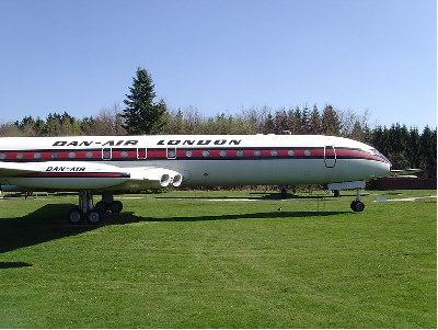
- In 1958 the company improved the Comet by releasing the generation 3 and 4, for which round glued windows and a thicker fuselage have been used, see Picture I.8. Unfortunately these models even though being very safe, never encountered a real commercial success.
- The systematic use of "Shot peening" for structures having to sustain a high number of cycles. This method consists in bombarding a surface by small spherical media. Those media introduce a residual compression in the surface layer and thus prevent crack initiation. The other technic is to polish a surface to remove initial micro-cracks.
- The consideration of the existing defects when predicting life and safety of the structure: this led to the development of the fracture mechanics analysis.