
Asymptotic Solution
This chapter details the steps required to establish the asymptotic solution in the LEFM context. Particular emphasis is put on the method applied and on the assumptions made.
Asymptotic Solution > Notations and assumptions
Linear elastic fracture mechanics consists in solving crack problems using classical linear elastic continuum mechanics.
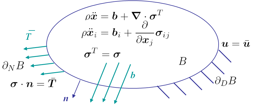
A body $B$ is balanced if the linear (translation) and angular (rotation) equilibrium equations, see Picture II.1, are satisfied. This problem is completed by the Dirichlet boundary conditions, which in our case means constrained displacements on $\partial_D B$, and by the Neumann boundary conditions, which correspond to constrained surface tractions on the surface $\partial_N B$.
We also assume that the body is submitted to small deformations, which means that the strain state $\mathbf{\varepsilon}$ can be derived from the displacements field $\mathbf{u}$ as follows:
\begin{equation} \mathbf{\varepsilon} = \frac{1}{2}\left(\nabla\otimes\mathbf{u}+\mathbf{u}\otimes\nabla\right). \label{eq:deformations}\end{equation}
In the indicial form, this equation reads:
\begin{equation}
\mathbf{\varepsilon}_{ij} = \frac{1}{2}\left(\frac{\partial}{\partial {x}_i}\mathbf{u}_j+\frac{\partial}{\partial {x}_j}\mathbf{u}_i\right),
\end{equation}
or again
\begin{equation} \mathbf{\varepsilon}_{ij} = \frac{1}{2}\left(\mathbf{u}_{j,i}+\mathbf{u}_{i,j}\right). \end{equation}
LEFM also assumes that the material is homogenous, isotopic and linear. The Hooke's law of the material relates the stress tensor $\mathbf{\sigma}$ to the strain tensor $\mathbf{\varepsilon}$:
\begin{equation} \mathbf{\sigma}=\mathcal{H}:\mathbf{\varepsilon}, \label{eq:Hooke}\end{equation}
or in the indicial form (with the summation on repeated indices)
\begin{equation} \sigma_{ij}=\mathcal{H}_{ijkl}\varepsilon_{kl}, \end{equation}
where the fourth-order tensor $\mathcal{H}$ is given by
\begin{equation} \mathcal{H}_{ijkl}=\frac{E\nu}{\left(1+\nu\right)\left(1-2\nu\right)}\delta_{ij}\delta_{kl} + \frac{E}{1+\nu}\left(\frac{1}{2}\delta_{ik}\delta_{jl}+\frac{1}{2}\delta_{il}\delta_{jk}\right). \end{equation}
The inverse law is simply given by:
\begin{equation} \mathbf{\varepsilon}=\mathcal{G} : \mathbf{\sigma}. \end{equation}
Using these notations and assumptions we are now able to determine the asymptotic solution at the crack tip. The range of validity of the LEFM approach will be determined in another lecture.
![]()