Fracture Mechanics Online Class

HRR theory

This chapter covers the HRR theory which was derived by Hutchinson, Rice and Rosengren in 1967-1968. The HRR theory allows evaluating the stress and displacement field of a stationary crack tip in the context of non-linear material behavior. Although the theory is formally only valid for crack initiation and not crack propagation, it is of great value since it provides an asymptotic solution for the stress and displacement field in the plastic zone near the crack tip where LEFM is not valid.

HRR theory > Elastoplastic behavior (continuation)

The understanding of elastoplastic behavior is essential for the HRR theory. Therefore, the related theory in the beforehand chapter is still valid and the reader is advised to review it if necessary.

HRR theory > General solution of the $J$-integral from near-tip fields

Assumptions and definitions

The HRR theory was developed for a semi-infinite crack, and is only valid up to crack initiation caused by a monotonic and proportionally increasing load, which means that all the stress tensor components should increase similarly. As a result of these assumptions, we can define an internal potential, see previous chapter. In addition, we consider the power hardening law, but in order to simplify the derivation, we assume that the elastic deformations can be neglected.

Since elastic deformations are neglected, the hardening power law is rewritten in terms of the equivalent von Mises stress and of the equivalent strain, which respectively read

\begin{equation} \sigma_e = \sqrt{\frac{3}{2} \mathbf{s}:\mathbf{s}} ,\label{eq:vmstress} \end{equation}

\begin{equation} \bar{\varepsilon} = \sqrt{\frac{2}{3} \strain:\strain}. \label{eq:vmstrain} \end{equation}

The hardening power law thus becomes

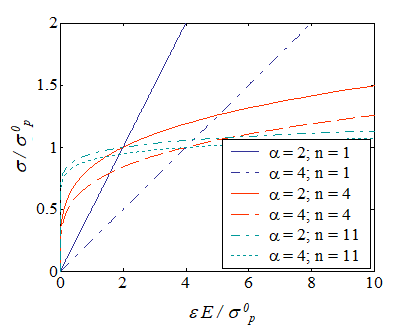
\begin{equation} {\sigma}_e \left(\bar{\varepsilon}\right) = {\sigma}_p^0{\left(\frac{\bar{\varepsilon}}{\frac{{\alpha}{\sigma}_p^0}{E}}\right)}^\frac{1}{n},\label{eq:elpowerlaw} \end{equation}

and governs the evolution of the equivalent von Mises stress in terms of the equivalent strain, below and above the yield stress ${\sigma}_p^0$. This law can be interpreted as a non-linear elastic law for isochoric solids. Indeed, since the elastic deformations are neglected, the whole deformation tensor $\strain$ is deviatoric. This non-linear elastic law is characterized by the parameters $\alpha$ and $n$ whose variations lead to different material responses as shown in Picture VIII.1. In particular, when $n\rightarrow\infty$, respectively $n\rightarrow 1$, a perfectly plastic-like, respectively linear, behavior is recovered.

The relation (\ref{eq:elpowerlaw}) can be inverted in order to express the evolution of the equivalent strain $\bar{\varepsilon}$ in terms of the von Mises stress ${\sigma}_e$, with

\begin{equation} \bar{\varepsilon}={\frac{{\alpha}{\mathbf{\sigma}_p^0}}{E}}{\left(\frac{{\sigma}_e}{{\sigma}_p^0}\right)}^n.\label{eq:elpowerlawinverted} \end{equation}

In order to investigate the evolution of the strain tensor $\mathbf{\varepsilon}$, the elastic power law (\ref{eq:elpowerlawinverted}) is first differentiated, leading to

\begin{equation} d\bar{\varepsilon}=\frac{n{\alpha}{\sigma}_p^0}{E} {\left(\frac{{\sigma}_e}{{\sigma}_p^0}\right)}^{n-1} \frac{d{\sigma}_e}{{\sigma}_p^0}\label{eq:derivationelpowerlaw1}, \end{equation}

which allows the plastic flow to be rewritten, with $\strain^\text{p}=\strain$ as

\begin{equation} d\strain=\sqrt{\frac{3}{2}}\frac{\mathbf{s}}{\sqrt{\mathbf{s}:\mathbf{s}}}\frac{n{\alpha}{\sigma}_p^0}{E}{\left(\frac{{\sigma}_e}{{\sigma}_p^0}\right)}^{n-1}\frac{d{\sigma}_e}{{\sigma}_p^0}=
\frac{3}{2}\frac{\mathbf{s}}{{\sigma}_p^0}\frac{n{\alpha}{\sigma}_p^0}{E}{\left(\frac{{\sigma}_e}{{\sigma}_p^0}\right)}^{n-2}\frac{d{\sigma}_e}{{\sigma}_p^0} . \label{eq:derivationelpowerlaw2}\end{equation}

Since the loading conditions are monotonic and proportional, the incremental form can be substituted by the finite one and the plastic strain tensor is directly obtained by combining the plastic flow, Eq. (\ref{eq:vmstress}) and Eq. (\ref{eq:elpowerlawinverted}) as,

\begin{equation} \strain=\bar{\varepsilon}\sqrt{\frac{3}{2}}\frac{\mathbf{s}}{\sqrt{\mathbf{s}:\mathbf{s}}}=
\left[\frac{{\alpha}{\sigma}_p^0}{E}{\left(\frac{{\sigma}_e}{{\sigma}_p^0}\right)}^n\right]
\sqrt{\frac{3}{2}}\frac{\mathbf{s}}{\sqrt{\mathbf{s}:\mathbf{s}}}=\left[\frac{{\alpha}{\sigma}_p^0}{E}{\left(\frac{{\sigma}_e}{{\sigma}_p^0}\right)}^{n-1}\right]\frac{3}{2}\frac{\mathbf{s}}{{\sigma}_p^0} . \label{eq:derivationelpowerlaw4}\end{equation}

\begin{equation} U=\int_0^{\strain}\cauchy:d\strain'=\int_0^{\strain}\mathbf{s}:d\strain',\label{eq:derivationelpowerlaw5} \end{equation}

since the deformation tensor is deviatoric. Using Eq. (\ref{eq:derivationelpowerlaw2}), Eq. (\ref{eq:vmstress}), and Eq. (\ref{eq:elpowerlaw}), this last relation reads

\begin{equation} U=\int_{0}^{{\sigma}_e} \mathbf{s}:\frac{3}{2}\frac{\mathbf{s}}{{\sigma}_p^0}\frac{n{\alpha}{\sigma}_p^0}{E}\left(\frac{{\sigma}_e'}{{\sigma}_p^0}\right)^{n-2}\frac{d{\sigma}_e'}{{\sigma}_p^0}=\int_{0}^{{\sigma}_e}\frac{n{\alpha}{\sigma}_p^0}{E}{\left(\frac{{\sigma}'_e}{{\sigma}_p^0}\right)}^n d{\sigma}'_e=\frac{n{\alpha}\left({\sigma}_p^0\right)^2}{E\left(n+1\right)}{\left(\frac{\bar{\varepsilon}}{{\frac{{\alpha}{\sigma}_p^0}{E}}}\right)}^\frac{n+1}{n}. \label{eq:derivationpowerlaw7}\end{equation}

Near-tip fields

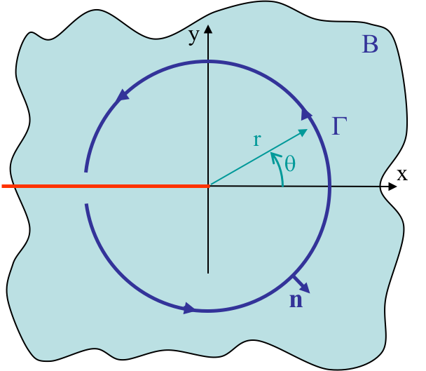
Since the $J$-Integral is path-independent, see related Chapter 3, one can consider as contour a circle of radius $r\rightarrow 0$ around the semi-infinite crack tip as depicted in Picture VIII.2, leading to the expression

\begin{equation} J=\lim_{r\rightarrow 0} \int_{-\pi}^{\pi} \left(U \uV{n}_x - \defu_{,x}\cdot \cauchy\cdot \uV{n}\right) r d\theta. \label{eq:JHRR} \end{equation}

Due to the path-independence of $J$, and thus the independence with respect to small $r$, the integrant of this last equation should only depend on $\theta$, yielding

\begin{equation} \lim_{r\rightarrow 0} \left(U \uV{n}_x - \defu_{,x}\cdot \cauchy\cdot \uV{n}\right) = \frac{h\left(\theta\right)}{r}.\label{eq:integrantHRR} \end{equation}

However, since the energy $U$ and the term $\defu_{,x}\cdot \cauchy$ involve products between strain and stress, Eq. (\ref{eq:integrantHRR}) is equivalent to

\begin{equation} \lim_{r\rightarrow 0} \cauchy : \strain = \frac{l\left(\theta\right)}{r}.\label{eq:integrant2HRR} \end{equation}

In the latter expressions, $h\left(\theta\right)$ and $l\left(\theta\right)$ are still unknown, but depend on $\theta$ and not on $r$. In order to evaluate them, the stress tensor is expanded in a power series

\begin{equation}\label{eq:constant_J} \cauchy\left(r,\,\theta\right) = \sum_s r^s \hat{\cauchy}\left(\theta,\,s\right) \,, \end{equation}

in which the tensors $\hat{\cauchy}\left(\theta,\,s\right)$, one different tensor for each term $s$ of the series, represents the distribution of the different stress components in terms of $\theta$. They are thus not depending on $r$.

Since we are trying to establish a relation in the vicinity of the crack tip, let $s'$ be the exponent corresponding to the dominant term near the crack tip. Therefore in the vicinity of the crack tip Eq. (\ref{eq:constant_J}) can be approximated by

\begin{equation}\label{eq:approx_stress_1} \cauchy \simeq r^{s'} \hat{\cauchy}\left(\theta,\,s'\right). \end{equation}

The approximated expressions of the deviatoric stress tensor $\mathbf{s}$ and of the equivalent von Mises stress $\sigma_e$ (\ref{eq:vmstress}) follow from

\begin{equation} \uT{s}\simeq r^{s'} \left(\hat{\cauchy}\left(\theta,\,s'\right)-\frac{\text{tr}\left(\hat{\cauchy}\left(\theta,\,s'\right)\right)}{3}\uT{I}\right) \,, \label{eq:approx_s_1} \end{equation}

\begin{equation} \sigma_e\simeq r^{s'}\sqrt{\frac{3}{2} \left(\hat{\cauchy}\left(\theta,\,s'\right)-\frac{\text{tr}\left(\hat{\cauchy}\left(\theta,\,s'\right)\right)}{3}\uT{I}\right): \left(\hat{\cauchy}\left(\theta,\,s'\right)-\frac{\text{tr}\left(\hat{\cauchy}\left(\theta,\,s'\right)\right)}{3}\uT{I}\right) },\label{eq:approx_svm_1} \end{equation}

Using these approximations, the strain tensor (\ref{eq:derivationelpowerlaw4}) becomes

\begin{equation} \strain \simeq \frac{\alpha\sigma_p^0}{E}\left(\frac{\sigma_e}{\sigma_p^0}\right)^{n-1}\frac{3\uT{s}}{2\sigma_p^0}= \left(r^{s'}\right)^{n}\hat{\strain}\left(\theta,\,s'\right) \, \text{.} \label{eq:approx_strain_1}\end{equation}

where the tensor $\hat{\strain}\left(\theta,\,s'\right)$ represents the distribution of the different strain components in terms of $\theta$ for the term $s'$ of the series (\ref{eq:constant_J}). Note that if $\hat{\cauchy}\left(\theta,\,s'\right)$ is known, the term $\hat{\strain}\left(\theta,\,s'\right)$ can readily be evaluated from (\ref{eq:approx_strain_1}).

Now, in order to satisfy the condition (\ref{eq:integrant2HRR}), by considering Eq. (\ref{eq:approx_stress_1}) and Eq. (\ref{eq:approx_strain_1}), it appears that the exponent $s'$ should be such that $s'n+s'=-1$, or in other words

\begin{equation}\label{eq:approx_exp} s' = \frac{-1}{n+1}. \end{equation}

The approximation of the stress field near the crack tip is thus obtained by inserting (\ref{eq:approx_exp}) into (\ref{eq:approx_stress_1}), leading to $\cauchy\left(r,\,\theta\right) \simeq r^{\frac{-1}{n+1}} \hat{\cauchy}\left(\theta,\, \frac{-1}{n+1}\right)$. However, since the stress tensor also depends on the loading condition and on the yield stress $\sigma_p^0$, in order to define the distribution of the different stress components in terms of $\theta$ (and the exponent $n$) only, we extract the loading and material effects from $\hat{\cauchy}\left(\theta,\,\frac{-1}{n+1}\right)$, resulting into

\begin{equation}\label{eq:J_stress} \cauchy\left(r,\,\theta\right) \simeq \sigma_p^0 k_n\frac{\tilde{\cauchy}\left(\theta,\,n\right)}{r^\frac{1}{n+1}}\,, \end{equation}

where $k_n$ is a plastic stress intensity factor, which depends on the geometry and loading conditions, and $\tilde{\cauchy}\left(\theta,\,n\right)$ is the distribution of the different stress components in terms of $\theta$ independently of the loading amplitude.

A similar procedure as to derive Eq. (\ref{eq:approx_strain_1}) can be applied for the stress tensor $\strain$, which leads to \begin{equation} \strain\left(r,\,\theta\right) \simeq \frac{\alpha\sigma_p^0}{E} \frac{k_n^n}{r^\frac{n}{n+1}}\tilde{\strain}\left(\theta,\,n\right)\,,\label{eq:J_strain} \end{equation}

where the tensor $\tilde{\strain}\left(\theta,\,n\right)$ represents the distribution of the different strain components independently of the loading amplitude and could be directly obtained from $\tilde{\cauchy}\left(\theta,\,n\right)$ (if it were known) through Eq. (\ref{eq:derivationelpowerlaw4}) as $\tilde{\strain}\left(\theta,\,n\right)=\frac{3}{2}\left(\sqrt{\frac{3}{2}\tilde{\uT{s}}:\tilde{\uT{s}}}\right)^{n-1}\tilde{\uT{s}}$, where $\tilde{\uT{s}}\left(\theta,\,n\right)=\tilde{\cauchy}\left(\theta,\,n\right)-\frac{\text{tr}\left(\tilde{\cauchy}\left(\theta,\,n\right)\right)}{3}\uT{I}$. Finally, the internal energy $U$ (\ref{eq:derivationpowerlaw7}) is approximated near the crack tip by

\begin{equation} U \simeq \label{eq:J_energy} \frac{n\alpha\left(\sigma_p^0\right)^2}{E\left(n+1\right)}\left(\frac{\sigma_e}{\sigma_p^0}\right)^{n+1}=\frac{n\alpha\left(\sigma_p^0\right)^2}{E\left(n+1 \right)} \frac{1}{r} k_n^{n+1}\sqrt{\frac{3}{2}\tilde{\uT{s}}:\tilde{\uT{s}} }^{n+1} \,, \end{equation}

where $\tilde{\uT{s}}$ could be directly obtained from $\tilde{\cauchy}\left(\theta,\,n\right)$ (if it were known).

Some remarks arise from this analysis:

Solution in terms of the J-integral

As previously stated, $k_n$ has been introduced to represent the dependency of the near-tip fields on the loading and geometry. However, the concept introduced in Chapter 3 to characterize the crack loading for non-linear behaviors is the $J$-Integral. We thus want to introduce this value in the asymptotic solution (\ref{eq:J_stress}-\ref{eq:J_energy}).

General stress and strain field

Using Eqs. (\ref{eq:J_stress}-\ref{eq:J_energy}) and assuming that the tensors components distributions, i.e. $\tilde{\cauchy}$, $\tilde{\strain}$ and $\tilde{\mathbf{s}}$, are known, the $J$ integral (\ref{eq:JHRR} ) is rewritten as

\begin{equation}\label{eq:Jint_rew_tmp} J=\lim_{r\rightarrow 0} \int_{-\pi}^{\pi} \left(U \uV{n}_x - \defu_{,x}\cdot \cauchy\cdot \uV{n}\right) r d\theta = \frac{\alpha\left(\sigma_p^0\right)^2}{E} k_n^{n+1} \int_{-\pi}^{\pi} \tilde{h} \left(\theta,\,n\right) d\theta \,, \end{equation}

where $\tilde{h} \left(\theta,\,n\right)$ gathers the terms in $\tilde{\cauchy} \left(\theta,\,n\right)$, $\tilde{\strain}$ and $\tilde{\mathbf{s}}$. Its expression will be discussed later. Therefore, Eq. (\ref{eq:Jint_rew_tmp}) is rewritten

\begin{equation}\label{eq:Jint_rew} J= \frac{\alpha\left(\sigma_p^0\right)^2}{E} k_n^{n+1} I_n\,, \end{equation}

with

\begin{equation} I_n = \int_{-\pi}^{\pi} \tilde{h} \left(\theta,\,n\right) d\theta\,,\label{eq:Jint_In} \end{equation}

which could be numerically evaluated from $\tilde{h} \left(\theta,\,n\right)$ if $\tilde{\cauchy} \left(\theta,\,n\right)$ were known. Eventually, solving (\ref{eq:Jint_rew}) for the plastic stress intensity factor $k_n$ with

\begin{equation} k_n = \left(\frac{J E}{\alpha\left(\sigma_p^0\right)^2I_n}\right)^{\frac{1}{n+1}} \, \text{,} \label{eq:Jint_kn}\end{equation}

we can calculate the stress (\ref{eq:J_stress}) and strain (\ref{eq:J_strain}) fields near the crack tip in a general form in terms of the $J$-integral through

\begin{equation}\label{eq:stress_Jint} \cauchy=\sigma_p^0\left(\frac{J E}{r\alpha\left(\sigma_p^0\right)^2I_n}\right)^{\frac{1}{n+1}}\tilde{\cauchy}\left(\theta,\,n\right), \end{equation}

\begin{equation}\label{eq:strain_Jint} \strain=\frac{\sigma_p^0\alpha}{E}\left(\frac{J E}{r\alpha\left(\sigma_p^0\right)^2I_n}\right)^{\frac{n}{n+1}} \tilde{\strain}\left(\theta,\,n\right) \end{equation}

As it can be deduced from (\ref{eq:stress_Jint}), the stress field near the crack tip is governed by $J$, which is the plastic analogue of the stress intensity factor $K$ in LFEM. The criterion for crack initiation should thus be written in terms of $J$ and may be $J \geq J_C$, where $J_C$ is a critical fracture energy. We can now consider two extreme cases:

Validity

The solution for the $J$-integral near the crack tip is not universal and only valid

Even though we have a solution for the stress and strain, two questions still remain unanswered:

Ludovic Noels, E-mail: L.Noels @ ulg.ac.be • University of Liège • Computational & Multiscale Mechanics of Materials (CM3)