Crack Growth > Stability
Considering a cracked body with $G \geqslant G_C$, then the crack propagates. However the crack can stop or not.
- If $G_C$ is constant, as for perfectly brittle materials, then there are two possible behaviors:
- $G$ decreases when the crack grows, and the crack could stop growing (unless the loading increases);
- $G$ increases or remains constant when the crack grows, and the behavior is unstable and leads to complete failure.
- If $G_C$ is not constant, meaning if $G_C$ increases with the crack size, the question to answer is which one of $G$ or $G_C$ grows at the highest rate.
As the stability depends on the evolutions of the energy release rate and of the fracture energy, a crack growth depends on the geometry, the loading and the material behavior.
Example: DCB specimen
Remember the case of the composite laminate delamination studied previously. In linear elasticity, the compliance and its derivative with respect to the crack surface $A=at$ read
\begin{equation} \begin{cases}C=\frac{u}{Q} = \frac{8 a^3}{Eth^3}\\ \partial_A C=\frac{1}{t}\partial_a \frac{8 a^3}{Eth^3} =\frac{24 a^2}{Et^2h^3}\end{cases}.\label{eq:CDCB}\end{equation}
Prescribed loading
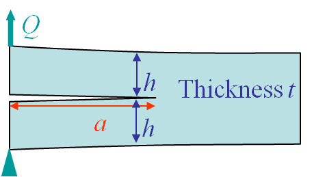
On the one hand if loading is prescribed, see Picture V.5, the energy release rate reads:
\begin{equation} G = \frac{Q^2}{2}\partial_A C = \frac{12Q^2a^2}{Et^2h^3}\label{eq:CDCBQ} \end{equation}
As the crack is growing, $G$ increases. For a perfectly brittle material, $G_C$ is constant, so the crack keeps propagating. This is an unstable crack.
Prescribed displacement
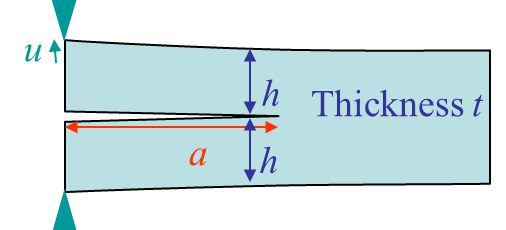
On the other hand, if the displacement is prescribed, see Picture V.6, the energy release rate reads:
\begin{equation} G = \frac{u^2}{2C^2}\partial_A C = \frac{3u^2Eh^3}{16a^4}\label{eq:CDCBu}. \end{equation}
As the crack is growing, $G$ decreases. For a perfectly brittle material, $G_C$ is constant, so at the some point the crack stops propagating. The crack is stable.
We have seen that for the DCB problem, a prescribed loading condition can lead to an unstable crack growth, while a prescribed displacement condition leads to a stable crack. But is it a general rule? What is happening for hyperstatic structures?
General loading conditions
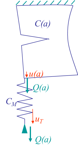
Practically structures are hyperstatic. This means that if a crack appears in a component, the compliance of this component increases (the stiffness decreases) and there is a new loading distribution in the structure. This means that the component with the crack is neither subject to a prescribed loading condition nor to a prescribed displacement condition, but to a mixed one. This can be modeled with the compliant machine, see Picture V.7, made of:
- A structure component with a crack of size $a$, and with a compliance $C\left(a\right)$;
- A spring of constant compliance $C_M$ modeling the remaining of the structure;
- A generalized loading $Q(a)$;
- A generalized displacement at the crack component $u(a)$;
- A prescribed displacement at one of the structure extremities $u_T$.
The displacements are defined as follows:
\begin{align} u_T & = Q(a) \left( C(a) + C_M \right) \\ u& = C(a) Q(a) = \frac{C(a)}{C(a) + C_M} u_T ,\end{align}
and the related internal energy becomes:
\begin{eqnarray} E_\text{int}&=&\frac{Qu}{2}+\frac{Q(u_T-u)}{2} \nonumber\\&=& \frac{C}{2(C+C_M)^2}u^2_T+\frac{C_M}{2(C+C_M)^2}u^2_T\nonumber\\&=&\frac{u_T^2}{2(C+C_M)}. \end{eqnarray}
From the previous relations, we can deduce the energy release rate:
\begin{equation} G = -\partial_A \left.E_\text{int}\right|_{u_T}= \frac{u_T^2}{2\left(C+C_M\right)^2} \partial_A C .\label{eq:complianceG}\end{equation}
The variation of this energy release rate with respect to the crack surface reads:
\begin{align} & \partial_A G = -\frac{u_T^2}{\left(C+C_M\right)^3} \left(\partial_A C\right)^2 + \frac{u_T^2}{2\left(C+C_M\right)^2} \partial^2_{AA} C \\ \Leftrightarrow & \partial_A G = - \frac{Q^2}{C+C_M} \left(\partial_A C\right)^2 + \frac{Q^2}{2} \partial^2_{AA} C . \label{eq:dAG}\end{align}
Dead load case
The dead load case (a constant load over time such as the structural weight itself) can be modeled with a spring of infinite compliance ($C_M \rightarrow \infty$). As the first term of (\ref{eq:dAG}) is negative, this value of $C_M \rightarrow \infty$ is the one for which $\partial_A G$ is maximum (as this cancels the negative first term), with
\begin{equation} \left.\partial_A G\right|_{\text{Dead load}}= \frac{Q^2}{2} \partial^2_{A^2} C.\label{eq:dAGDeadLoad} \end{equation}
Mixed case
As the spring stiffens toward a fixed grip, $C_M$ decreases and so does $\partial_A G$, which tends to stabilize the crack growth.
If $\partial_A G$ becomes negative, the crack becomes stable for a perfectly brittle material ($G_c$ is a constant).
Fixed grip case
The fixed grip case (a constant displacement $u$ over time) can be modeled with a spring of zero-compliance ($C_M \rightarrow 0$). In that case (\ref{eq:dAG}) is minimum and reads
\begin{equation} \left.\partial_A G\right|_{\text{Fixed grip}}= - \frac{Q^2}{C} \left(\partial_A C\right)^2 + \frac{Q^2}{2} \partial^2_{A^2} C = - \frac{u^2}{C^3} \left(\partial_A C\right)^2 + \frac{u^2}{2C^2} \partial^2_{A^2} C .\label{eq:dAGFixedGrip}\end{equation}
Note that a fixed grip is always more stable than a dead load as $ \partial_A G$ is smaller.
Resistance curve
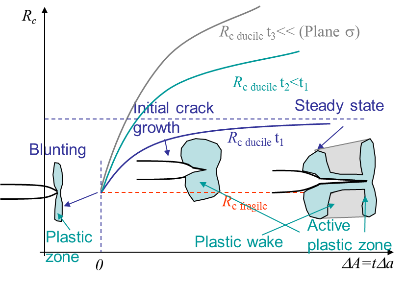
Remember we have already introduced the resistance curve. For a perfectly brittle material the fracture energy $G_C$ is constant and equal to $2\gamma_s$. For other materials there will be a plastic flow at the crack tip as a stress cannot physically reach the infinity as predicted by the LEFM approach. This plastic flow arises in the active plastic zone as illustrated in Picture V.8. Evidently this active plastic zone moves with the crack tip in case of crack growth, meaning that the crack is opening in a zone affected by permanent plastic deformations: the plastic wake. This makes the crack more difficult to be opened, which corresponds to an increase of the apparent fracture energy $G_C$ with the crack propagation $\Delta a$. This is call the resistance and $G_c$ is replaced by $R_c(a)$. Some material can have a steady-state in the resistance curve as in Picture V.8, other not. Note that the curve does not only depend on the material, but also on the geometry as the thickness.
So for non-perfectly brittle materials, a crack can be stable even if $\partial_A G > 0$ as $R_c$ also depends on the crack surface. In 2D, $R_c (\Delta A) = R_c (t \Delta a)$
Example: delamination of a composite with initial crack $a_0$
On the one hand, for composites, as the crack propagates, fibers in the wake tend to close the crack tip so more energy is required for the crack to grow, and we have a curve $R_c (t \Delta a)$. On the other hand, we have previously evaluated the energy release rate of the DCB problem from the compliance variation (\ref{eq:CDCB}). We can now study the stability of the delamination.
Prescribed loading
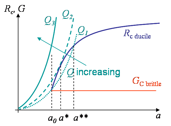
We have previously computed the shape of the energy release rate (\ref{eq:CDCBQ}) as being $G = \frac{Q^2}{2}\partial_A C = \frac{12Q^2a^2}{Et^2h^3}$. As the crack is growing, $G$ also increases, see Picture V.9. Let us consider different loading values:
-
Dead load $Q_1$: As $G=G_C$ for a crack size $a_0$, the crack propagated
- For a perfectly brittle materials $G$ remains larger than $G_C$ and the crack is unstable.
- For composites with a resistance curve, $R_c$ becomes larger than $G$ and the crack is stable. To increase the crack size we need to increase $Q$. However, if $a$ is larger than $a^{\star \star}$ it turns unstable even for $Q_1$.
- Dead load $Q_2 > Q_1$: This is the limit of stability for composites (always unstable for perfectly brittle material).
- For $Q_3> Q_2$: The crack is always unstable.
Prescribed displacement
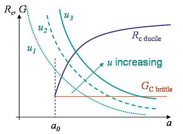
We have previously computed the shape of the energy release rate (\ref{eq:CDCBu}) as being $G = \frac{Q^2}{2}\partial_A C = \frac{3u^2Eh^3}{16a^4}$. As the crack is growing, $G$ decreases, see Picture V.10, contrarily to the dead load case. In this case, whatever the value $u$ of the grip and whatever the material, $G$ always becomes smaller than $G_C$ (or $R_c$) for a given crack size, and the crack stops. This is a stable configuration.
Summary
- The crack growth criterion is $G \geq G_c$.
- The crack growth is stable if, in 2D, $\partial_a G \leq \partial_a R_c$ and unstable otherwise.
In this part we have considered mode I failure. The case of mixed mode is considered in the next page.
![]()