Energetic Approach > The energy release rate
In the previous section we have deduced the energy released by the system when the crack surface increases and we have found
\begin{equation} G = \begin{cases} & - \partial_A \left( E_\text{int} - Q u\right) &\text { for a prescribed loading} \\ &- \partial_A E_\text{int} & \text { for a prescribed displacement}\end{cases}.\label{eq:GPrescribedCases}\end{equation}
Note that these equations hold for any elastic materials, linear or not. The only requirement is the existence of a material internal potential $U$. Nevertheless the expression of $G$ depends on the loading conditions, and one would like to define it for a general loading condition.
General Loading
Let us define the potential energy of the specimen as
\begin{equation}\Pi_T = E_\text{int}-W_{\text{ext}}.\label{eq:potEnergy}\end{equation}
The energy release rate is thus defined as the energy, per unit crack surface, released by the system assuming a crack grows
\begin{equation} G = -\partial_A \left(E_\text{int}-W_\text{ext}\right) = - \partial_A \Pi_T .\label{eq:G}\end{equation}
Note that in the case of prescribed loading or displacement, (\ref{eq:G}) simplifies into (\ref{eq:GPrescribedCases}).
Crack growth
What has to be understood from the definition of the energy release rate (\ref{eq:G}) is that the crack growth is purely virtual: We evaluate the energy released by the system if a crack would grow. But what is required for a crack to grow?
Let us now consider the total energy of the system
\begin{equation}E=\Pi_T + \Gamma,\label{eq:sysEnergy}\end{equation}
where $\Gamma$ is the energy required to create a crack surface $A$ in the body. Two kinds of materials can be considered
- For brittle materials the energy required to create a crack surface is the energy required to break the atomic bonds. So $\partial_A \Gamma= 2\gamma_s$, with $\gamma_s$ the surface energy of the material (a crack creates 2 surfaces, so the presence of the 2). This is a material constant that can be measured (with difficulties for solids however).
- For other materials (ductile, composite , polymers , etc) this energy depends on the failure process, void coalescence, debonding ... For ductile materials we need to consider the energy required for the plastic deformations precluding the crack formation and $\partial_A \Gamma= 2\gamma_s + W_\text{pl}$.
For both cases we define the fracture energy as the energy required to form a unit surface in the material
\begin{equation}G_C = \partial_A \Gamma.\label{eq:Gc}\end{equation}
As the derivation of (\ref{eq:sysEnergy}) implies
\begin{equation} \partial_A E= \partial_A \Pi_T +\partial_A \Gamma=G_C-G,\label{eq:dsysEnergy}\end{equation}
we have now a crack propagation criterion:
- If $G<G_C$ then $\partial_A E<0$, which is impossible. So the crack does not propagate as the energy released from the system potential energy is not enough to create the surface in the material.
- If $G>G_C$ then $\partial_A E>0$ and the crack propagates as the energy released by the system potential energy (internal energy and/or work of external forces) is enough to create a surface in the material.
Thus the crack propagation criterion simply reads
\begin{equation} G \begin{cases} & < G_C &\text { no propagation} \\ &\geq G_C & \text { propagation}\end{cases}.\label{eq:Gcriterion}\end{equation}
In this relation $G$ depends on the sample geometry (including crack length) and boundary conditions, while $G_C$ depends on the material (for ductile materials it can also depend on the crack advance).
We have now introduced the energy release rate concept and have related it to a fracture criterion. These considerations are valid for elastic materials (or materials that can be considered as it) as we have assumed a material internal potential $U$. We did not make assumption on the linearity or not of the elastic material. However, things become easier for linear elasticity.
Linear case and compliance
In particular, in linear elasticity the expression (\ref{eq:GPrescribedCases}) of $G$ for different loading conditions can be unified in terms of the structure compliance $C$. Indeed as the material is linear the compliance of the specimen, for a given crack surface $A$, is defined as
\begin{equation} C\left(A\right)=\frac{u}{Q}\label{eq:C}.\end{equation}
The system energies can directly be computed from this compliance
\begin{equation} \begin{cases} E_\text{int} &=& \frac{1}{2}Qu=\frac{u^2}{2C} = \frac{Q^2C}{2}\\ W_\text{ext} &=& Qu = \frac{u^2}{C}=Q^2C\end{cases}\label{eq:ELinear}.\end{equation}
We can now analyze the two cases of interest.
Prescribed displacements
In that case, (\ref{eq:GPrescribedCases}) simplifies into
\begin{equation} G =- \left.\partial_A E_\text{int}\right|_u = -\left.\partial_A \left(\frac{u^2}{2C}\right)\right|_u = \frac{u^2}{2C^2}\partial_AC = \frac{Q^2}{2}\partial_A C .\label{eq:GLinearPrescribedDisp}\end{equation}
The physical interpretations of this relation are
- For the crack to grow all the required energy comes from the elastic internal energy (as the external forces do not work).
- As a result the internal energy decreases with the crack growth.
Prescribed loading
In that case, (\ref{eq:GPrescribedCases}) simplifies into
\begin{equation} G =- \left.\partial_A \left(E_\text{int}-Q u\right)\right|_Q = -\left.\partial_A \left(\frac{Q^2C}{2}-Q^2C\right)\right|_Q = \frac{Q^2}{2}\partial_AC.\label{eq:GLinearPrescribedLoading}\end{equation}
This expression is similar as (\ref{eq:GLinearPrescribedDisp}) obtained for a prescribed displacement. However the implication is quite different. Indeed, starting again from (\ref{eq:GPrescribedCases}) and using (\ref{eq:GLinearPrescribedLoading}), we have
\begin{equation} \begin{cases} G =- \left.\partial_A \left(E_\text{int}-Q u\right)\right|_Q = -\left.\partial_A E_\text{int}\right|_Q + \left. \partial_A\left(Q
u\right)\right|_Q
\\ \iff G + \left.\partial_A E_\text{int}\right|_Q = Q \partial_A u =
Q^2\partial_AC = 2G\\\iff G =\left.\partial_A E_\text{int}\right|_Q\end{cases}
.\label{eq:GLinearPrescribedLoading1}\end{equation}
The physical interpretations of this relation are
- For a crack to grow of $dA$, the external forces have to achieve a work of $2G$ as the internal energy is also increased by $G$.
- The internal energy increases with the crack growth contrarily to the prescribed displacement case.
Application of the compliance method: Delamination of a composite laminate
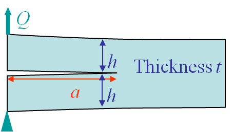
Delamination is a common failure mode in composite structures. The composite laminate is made of a stacking sequence of composite plies and two plies can unglue from each other due to the shear force, leading to delamination. This effect can be modeled by considering two clamped beams as in Picture III.10. This model is valid when the crack is long compared to the ply thickness: $a>>>h$. In that case we can consider two identical (semi-)cantilever beams of length $a$. The question is how to determine the energy release rate of this structure.
The resolution method is as follows:
-
Usual beam theory predicts the displacement $u$ of the double system from the deflection $v_\text{max}$ of a beam subjected to an end load $Q$.:\begin{equation} \begin{cases} v_\text{max}= \frac{Qa^3}{3EI} \text{ with }
I = \frac{t h^3}{12}\\
\iff u=2 v_\text{max} = \frac{8Q a^3}{Eth^3}\end{cases} \label{uDCB}. \end{equation} - The compliance and its derivative with respect to the crack surface $A=at$ can directly be evaluated from this last expression \begin{equation} \begin{cases}C=\frac{u}{Q} = \frac{8 a^3}{Eth^3}\\ \partial_A C=\frac{1}{t}\partial_a \frac{8 a^3}{Eth^3} =\frac{24 a^2}{Et^2h^3}\end{cases}.\label{eq:CDCB}\end{equation}
- Using (\ref{eq:ELinear}) the energy release rate reads \begin{equation}G=\frac{Q^2}{2}\partial_A C=\frac{12 Q^2 a^2}{Et^2h^3} . \label{eq:GDCB}\end{equation}
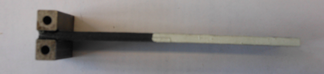
This model can be used to measure the delamination energy of composite plies following a rigorous standard (ISO 15024). This process is summarized by
- A sample is manufactured with two plies partially unglued (use of a tape between the plies during manufacturing). Two loading blocks are glued on the resulting beams, see Picture III.11.
- A crack is then initiated between the plies from the originally unglued part by applying a first loading/unloading cycle.
- The length of the resulting crack is then deduced from the unloading response using (\ref{eq:CDCB}).
- A second loading is then applied and the maximum force reached before the stable crack propagation is used to determine the initiation $G_C$ from a corrected expression of (\ref{eq:GDCB}).
- To differentiate the initiation $G_C$ and the propagation one, the value $G_C(a)$ can be monitored with the crack propagation length.
![]()