Energetic Approach > Crack closure integral
On the one hand, we have seen that the energy release rate $G$ is the variation of the system potential energy with respect to the crack size. Knowing the fracture energy required for acrack surface to form in a given material, this concept can be used to write a fracture criterion
\begin{equation} G \begin{cases} & < G_C &\text { no propagation} \\ &\geq G_C & \text { propagation}\end{cases}.\label{eq:Gcriterion}\end{equation}
In this relation $G$ depends on the sample geometry (including crack length) and on the boundary conditions, while $G_C$ depends on the material (for ductile materials it can also depend on the crack advance). The concept of energy release rate $G$ is based on the existence of an internal material potential, and thus on elasticity, but does not require linear material behaviors.
On the other hand we have seen previously that for linear elasticity that in 1957 G. R. Irwin introduced a new failure criterion using the SIFs defined in the asymptotic solution. In mode I this criterion reads
\begin{equation}K_I\quad\begin{cases} < K_{IC} \rightarrow \text{ the crack does not propagate,}\\ \geq K_{IC} \rightarrow \text{ the crack does propagate,} \end{cases}\label{eq:SIFCriterion}\end{equation}
where $K_{IC}$ is the mode I toughness. Under the LEFM assumption:
- $K_I$ depends on the geometry and loading conditions only,
- $K_{IC}$ depends on the material only.
We have thus two concepts, energy and SIFs, which should give the same predictions when both are valid: in linear elasticity. In this section we establish the relation between the energy release rate and the SIFs.
Notations
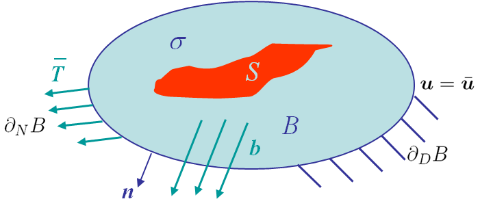
In 1957 Irwin introduced the crack closure integral. We use the notations and governing equations previously detailed. The difference lies in the presence of an initial cavity of surface $S$ in the body B, as illustrated in Picture III.12. In this initial configuration the following assumptions are made:
- The stress state is $\mathbf{\sigma}$;
- The displacement fields is $\mathbf{u}$ (in $B$ and on $S$) and is constrained to $\bar{\mathbf{u}}$ on $\partial_D B$;
- The surface traction is $\mathbf{T}$ with the constraints $\bar{\mathbf{T}}$ on $\partial_N B$, and $0$ on $S$ (stress free cavity surface).
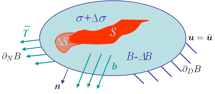
Then, the cavity is assumed to grow to $S+\Delta S$ leading to a final configuration, with
- A volume loss of $\Delta B$;
- The stress state becoming $\mathbf{\sigma}+\Delta\mathbf{\sigma}$;
- The displacement field becoming $\mathbf{u}+\Delta\mathbf{u}$ with $\Delta \mathbf{u} = 0$ on $\partial_D B$;
- The surface traction becoming $\mathbf{T}+\Delta\mathbf{T}$ with $\Delta \mathbf{T} = 0$ on $\partial_N B$ and $0$ on $S+\Delta S$.
Potential energy
In elasticity (linear or non-linear) there exists a material internal potential $U$, which depends on the strain state. As the strain depends on $\mathbf{\nabla}\mathbf{u}$, we can use the notation $U\left(\mathbf{\nabla}\mathbf{u}\right)$ and if $b$ is assumed equal to 0, the potential energy can be obtained for the two configurations as
\begin{equation}
\begin{cases} \Pi_T& = &\int_B U\left(\mathbf{\nabla}\mathbf{u}\right) dB - \int_{\partial_NB} \bar{\mathbf{T}} \cdot \mathbf{u} d\partial B\\
\Pi_T+\Delta \Pi_T &=& \int_{B-\Delta B} U\left(\mathbf{\nabla}\mathbf{u}+\mathbf{\nabla}\Delta\mathbf{u}\right) dB - \int_{\partial_N B} \bar{\mathbf{T}} \cdot \left(\mathbf{u}+\Delta\mathbf{u}\right) d\partial B\end{cases}.\label{eq:piCCI} \end{equation}
The difference of the potential energies between the two configurations reads
\begin{equation} \Delta \Pi_T = \int_{B-\Delta B} U\left(\mathbf{\nabla}\mathbf{u}+\mathbf{\nabla}\Delta\mathbf{u}\right)-U\left(\mathbf{\nabla}\mathbf{u}\right) dB-\int_{\Delta B} U\left(\mathbf{\nabla}\mathbf{u}\right) dB - \int_{\partial_N B} \bar{\mathbf{T}} \cdot\Delta\mathbf{u}d\partial B.\label{eq:DpiCCI1} \end{equation}
As by definition $\mathbf{\sigma}=\partial_{\mathbf{\varepsilon}} U$, the first term of the right hand side of (\ref{eq:DpiCCI1}) can be rewritten
\begin{eqnarray}\int_{B-\Delta B} U\left(\mathbf{\nabla}\mathbf{u}+\mathbf{\nabla}\Delta\mathbf{u}\right)-U\left(\mathbf{\nabla}\mathbf{u}\right) dB &=&\int_{B-\Delta B} U\left(\mathbf{\varepsilon}+\Delta\mathbf{\varepsilon}\right)-U\left(\mathbf{\varepsilon}\right) dB \nonumber \\ &=& \int_{B - \Delta B}\left\{ \int_0^{\mathbf{\varepsilon}+\Delta\mathbf{\varepsilon}}\mathbf{\sigma}\left(\mathbf{\varepsilon}'\right):
d\mathbf{\varepsilon}' -\int_0^{\mathbf{\varepsilon}}\mathbf{\sigma}\left(\mathbf{\varepsilon}'\right): d\mathbf{\varepsilon}'\right\} dB,
\end{eqnarray}
which simplifies into
\begin{equation}\int_{B-\Delta B} U\left(\mathbf{\nabla}\mathbf{u}+\mathbf{\nabla}\Delta\mathbf{u}\right)-U\left(\mathbf{\nabla}\mathbf{u}\right) dB = \int_{B - \Delta B} \int_\mathbf{\varepsilon}^{\mathbf{\varepsilon}+\Delta\mathbf{\varepsilon}}\mathbf{\sigma}\left(\mathbf{\varepsilon}'\right):
d\mathbf{\varepsilon}' dB\label{eq:DpiCCItmp}.
\end{equation}
As $ \mathbf{\sigma}$ is symmetric, we have $ \mathbf{\sigma}\left(\mathbf{\varepsilon}'\right):
d\mathbf{\varepsilon}'=\mathbf{\sigma}\left(\mathbf{\varepsilon}'\right):
\mathbf{\nabla}d\mathbf{u}'=\mathbf{\nabla} \cdot\left(\mathbf{\sigma}^T\cdot d\mathbf{u}'\right)-\left(\mathbf{\nabla} \cdot\mathbf{\sigma}^T\right)\cdot d\mathbf{u}'$. As $\mathbf{b}=0$, the linear momentum equation implies $\mathbf{\nabla} \cdot\mathbf{\sigma}^T=0$ and (\ref{eq:DpiCCItmp}) becomes
\begin{eqnarray}
\int_{B-\Delta B} U\left(\mathbf{\nabla}\mathbf{u}+\mathbf{\nabla}\Delta\mathbf{u}\right)-U\left(\mathbf{\nabla}\mathbf{u}\right) dB &= & \int_{B -
\Delta B}\int_{\mathbf{u}}^{\mathbf{u}+\Delta\mathbf{u}}\mathbf{\nabla}\cdot\left(
\mathbf{\sigma}^T\left(\mathbf{u}'\right)\cdot d \mathbf{u}'\right) dB
\nonumber\\&=& \int_{S+ \Delta S+\partial_N B+\partial_D B}\int_{\mathbf{u}}^{\mathbf{u}+\Delta\mathbf{u}}
\left[\mathbf{\sigma}\left(\mathbf{u}'\right) \cdot \mathbf{n}\right]\cdot d \mathbf{u}' d\partial B,\label{eq:DpiCCItmp2}\end{eqnarray}
where we have applied Gauss theorem. From our assumptions
- The surface traction $\bar{\mathbf{T}}$ is constant on $\partial_N B$ and the displacement is constant on $\partial_D B$ ($d\mathbf{u}=0$);
- On the cavity surface $S$(+$\Delta S$), the surface traction $t$ is defined as $\mathbf{\sigma} \cdot \mathbf{n}$.
Then (\ref{eq:DpiCCItmp2}) becomes
\begin{equation} \int_{B-\Delta B} U\left(\mathbf{\nabla}\mathbf{u}+\mathbf{\nabla}\Delta\mathbf{u}\right)-U\left(\mathbf{\nabla}\mathbf{u}\right) dB = \int_{S+ \Delta S}\int_{\mathbf{u}}^{\mathbf{u}+\Delta\mathbf{u}} \mathbf{t}\left(\mathbf{u}'\right)\cdot d \mathbf{u}' d\partial B+ \int_{\partial_NB}
\bar{\mathbf{T}}\cdot\Delta \mathbf{u} d\partial B.\label{eq:DpiCCItmp3}\end{equation}
Here we need to discuss the stress-free nature of the cavity surface.
- The final cavity surface $S+\Delta S$ is stress-free, but only in the final configuration, so $\mathbf{\sigma}\left(\mathbf{u}+\Delta\mathbf{u}\right)\cdot\mathbf{n}=0$ on $S+\Delta S$;
- The surface $S$ corresponding to the initial cavity remains stress-free during the whole process, so $\mathbf{\sigma}\left(\mathbf{u}'\right)\cdot\mathbf{n}=0$ on $S$;
- During the cavity growth process there is a surface traction on $\Delta S$ as the cavity is not formed yet, so $\mathbf{\sigma}\left(\mathbf{u}'\right)\cdot\mathbf{n}\neq 0$ on $\Delta S$.
Because of these considerations, (\ref{eq:DpiCCItmp3}) is finally rewritten
\begin{equation} \int_{B-\Delta B} U\left(\mathbf{\nabla}\mathbf{u}+\mathbf{\nabla}\Delta\mathbf{u}\right)-U\left(\mathbf{\nabla}\mathbf{u}\right) dB = \int_{\Delta S}\int_{\mathbf{u}}^{\mathbf{u}+\Delta\mathbf{u}} \mathbf{t}\left(\mathbf{u}'\right)\cdot d \mathbf{u}' d\partial B+ \int_{\partial_NB}
\bar{\mathbf{T}}\cdot\Delta \mathbf{u} d\partial B.\label{eq:DpiCCItmp4}\end{equation}
Using this last result, the change of potential energy (\ref{eq:DpiCCI1}) reads
\begin{equation} \Delta \Pi_T = \int_{\Delta S}\int_{\mathbf{u}}^{\mathbf{u}+\Delta\mathbf{u}} \mathbf{t}\left(\mathbf{u}'\right)\cdot d \mathbf{u}' d\partial B - \int_{\Delta B} U\left(\mathbf{\nabla}\mathbf{u}\right) dB.\label{eq:DpiCCI2} \end{equation}
As instead of a cavity we consider a crack, the change of volume vanishes and we eventually have
\begin{equation} \Delta \Pi_T = \int_{\Delta S}\int_{\mathbf{u}}^{\mathbf{u}+\Delta\mathbf{u}} \mathbf{t}\left(\mathbf{u}'\right)\cdot d \mathbf{u}' d\partial B .\label{eq:DpiCCI} \end{equation}
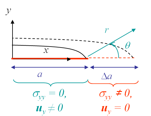
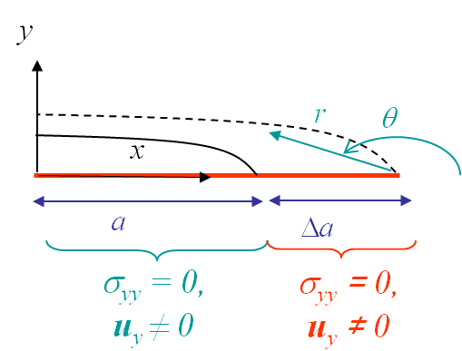
As explained in the overview, the physical interpretation of (\ref{eq:DpiCCI}) can be explained by considering a crack growth from a size $2a$, see Picture III.14, to a size $2(a+\Delta a)$, see Picture III.15, of a centered crack in an infinite plate. During this crack propagation, $\sigma_{yy}$ produces a (negative) work on the crack growth $\Delta a$.
Energy release rate in linear elasticity
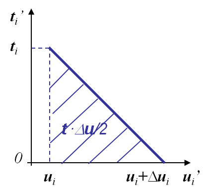
The general expression of the change of potential energy (\ref{eq:DpiCCI}) is valid in the general elastic case (linear or not). If the response is elastic and linear, see Picture III.16, this expression can be evaluated as
- The traction $t'$ is decreasing linearly with $u'$ (linear material response);
- The achieved work is then $t \frac{\Delta u}{2}$.
The variation of potential of potential energy (\ref{eq:DpiCCI}) now reads
\begin{equation} \Delta \Pi_T = \int_{\Delta S}\frac{1}{2} \mathbf{t}\cdot \Delta \mathbf{u} d\partial B, \label{eq:DpiCCILin} \end{equation}
where
- $\mathbf{t}$ is the tension before crack propagation and where, see Picture III.16,
- $\Delta \mathbf{u}$ is the opening after crack propagation, see Picture III.16.

To evaluate the energy release rate, we need to relate (\ref{eq:DpiCCILin}) with the increment of crack surface. The created surface $\Delta S$ has actually two sides: an upper side $\Delta A^+$ and a lower side $\Delta A^-$, with $\left.\mathbf{t}\right|_{\Delta A^+} = -\left.\mathbf{t}\right|_{\Delta A^-}$ by action-reaction, and with the notation $\left.\Delta\mathbf{u}\right|_{\Delta A^\pm} = \Delta\mathbf{u}^\pm$. Hence (\ref{eq:DpiCCILin}) is rewritten
\begin{eqnarray} \Delta \Pi_T &=& \int_{\Delta A^+}\frac{1}{2} \mathbf{t}\cdot \left[\Delta \mathbf{u}^+ - \Delta \mathbf{u}^-\right]d\partial B\nonumber\\ &=& \int_{\Delta A^+}\frac{1}{2} \mathbf{t}\cdot [\![ \Delta \mathbf{u} ]\!] d\partial B, \end{eqnarray}
where $[\![ \Delta\mathbf{u}]\!]$ is the opening between the crack lips. The increment of fracture area $\Delta A$ corresponds to $\Delta A^+$, so that the energy release rate $G$ becomes:
\begin{equation} G= -\partial_A \Delta \Pi_T = - \lim_{\Delta A\rightarrow 0}\frac{1}{\Delta A} \int_{\Delta A}\frac{1}{2} \mathbf{t}\cdot [\![\Delta \mathbf{u} ]\!] d\partial B \label{Glin}. \end{equation}
This relation is valid for any linear elastic materials and for any directions of crack growth (mode I, II or III).
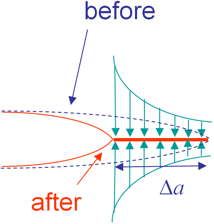
We can relate the expression (\ref{Glin}) to the work needed to close a crack. On the one hand, we know that $G > 0$ for a crack growth and from (\ref{Glin}) it appears that $\Pi_T$ decreases during the crack growth. This means the system free some energy which is used to break the bonding (or for plastic deformation etc). On the other hand, $G$ (\ref{Glin}) can also be interpreted as the energy required to close the crack tip on a surface $\Delta A$, with $\mathbf{t}$ the force required to close the opening $[\![\Delta \mathbf{u}]\!]$. Assuming a tensile mode I, this crack closure is illustrated in Picture III.18.
The next page particularies these expressions when cracks grow straight ahead.