In the previous section we have seen the effect of cracks on cleavage of brittle materials. However other modes of failure exist.
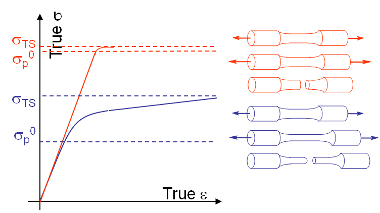
By definition samples made of a brittle material do not exhibit plastic deformations prior to their macroscopic failure (red curve on Picture I.21), contrarily to samples made of ductile materials (blue curve on Picture I.21). The shape of the fracture surface is also different.
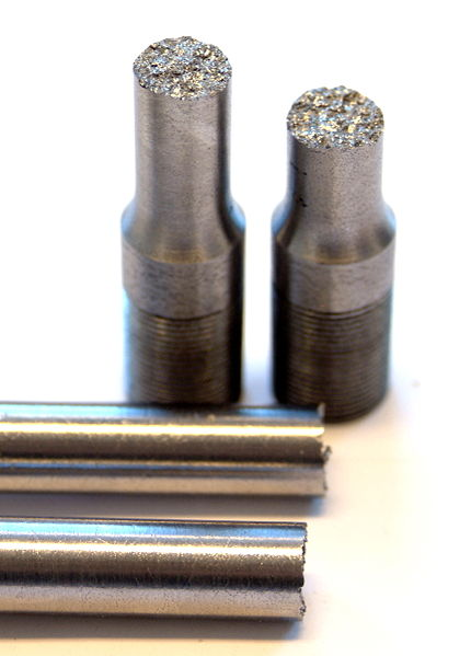
For a brittle fracture the fractured surface remains planar on average as shown in Picture I.22. When magnifying the fracture surface it appears that the failure occurred along the lattice planes by cleavage, i.e. by separation of crystallographic planes see Picture I.23. The cleavage happens within the grains in the case od intra-granular failure Note that under some circumstances like during creep, corrosion, presence of trapped H2.... the failure mode can become inter-granular at it will be discussed in another chapter.
For brittle materials Griffith law is valid:
\begin{equation} \sigma_{\text{TS}}\sqrt{a} \div \sqrt{E\, 2\gamma_s} \label{eq:griffith} \end{equation}
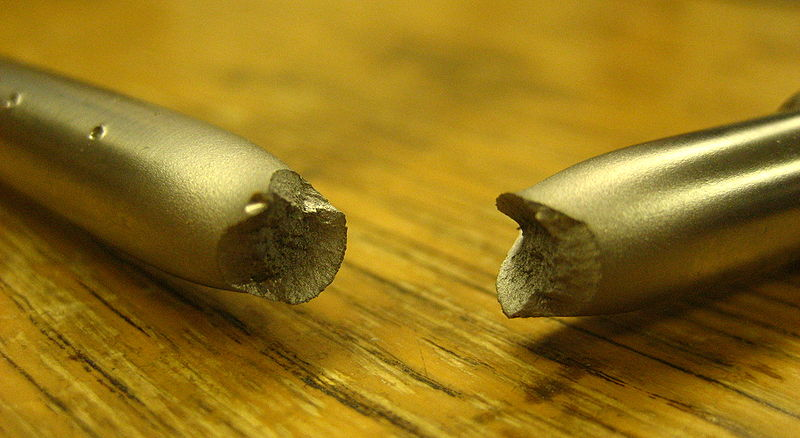
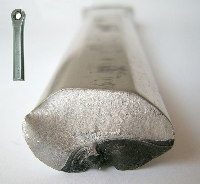
Contrarily to brittle materials, ductile materials exhibit plastic deformations prior to macroscopic failure. For a tensile test a macroscopic sample will exhibit necking before fracture, see Picture I.24. The fracture surface has also a different aspect: instead of being composed of crystallographic planes, the surface is rougher and exhibits small craters. This appearance can be explained by the existence of plastic deformations, which corresponds to the motion of dislocations. As dislocations are nothing else but missing atoms in the crystallographic organisation, they can be seen as voids. During the disclocations motion, these voids tend to gather together around obstacles which block their motion, as inclusions or grain boundaries, and to form micro-voids. These in turn leads to micro cavities coalescence and to crack growth, see Picture I.25.
For such materials the Griffith law cannot be applied but has to be modified. Irwin (1950) found that the plastic work at the crack tip should be added to the surface energy:
\begin{equation} \sigma_{\text{TS}}\sqrt{a} \div \sqrt{E\left(2\gamma_s+W_\text{pl}\right)} \label{eq:irwin} \end{equation}
The question is now, why does a material exhibit a brittle or ductile behavior? This will be explained by the failure induced mechanics at the micro-level in the next section. However note that another common fracture mode exists: fatigue, which also exhibits a different fracture surface as in Picture I.26. We will briefly introduce this point later on and will detail it in a coming section.
In order to predict the failure mode of a given material we first need to analyze the different deformation mechanisms involved at the atomic level.
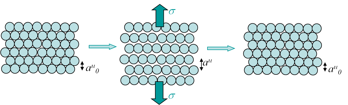
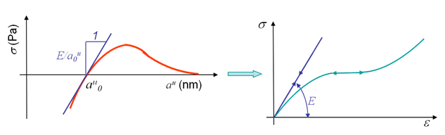
When submitted to small traction, most of the materials exhibit reversible deformations, meaning that once the stress is released the initial configuration is recovered. This is called elasticity and can be explained by the microscopic behavior illustrated in Picture I.27. As it can be seen, this elastic behavior is due to the stretching of bonds (Picture I.27, middle), which remains reversible for small stress (Picture I.27, right). The slope at the origin of the stress-strain curve, see Picture I.28 right, is the Young modulus $E$. This modulus can be deduced from the free electrons model by considering the slope of the function $\sigma(a^u)$, see Picture I.28 left, as explained in the previous section. Note that elasticity can be either linear (metals) or non-linear (polymers), see Picture I.28.
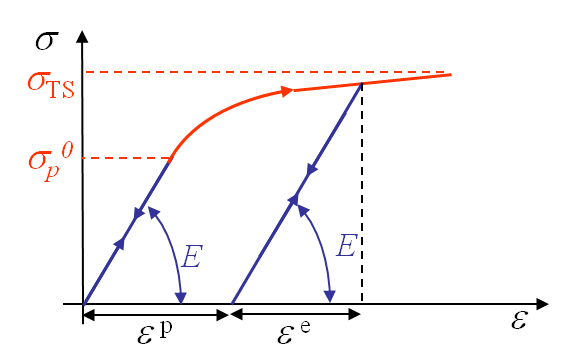
Some materials exhibit plastic deformation before fracture, see Picture I.29. Usually plasticity occurs above a given stress threshold: the yield stress. If the stress is then released, only a part of the deformations is recovered: the elastic part $\varepsilon^e$. A permanent deformation remains: the plastic deformation $\varepsilon^p$.
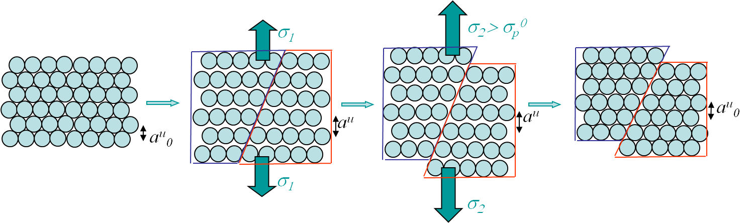
This elasto-plastic behavior can be explained at the microscopic level by the plane shearing mechanism illustrated in Picture I.30. At a first stage for $\sigma = \sigma_1$, only bonds stretching is involved and a pure elastic behavior is observed, see Picture I.30 center-left . However for a higher stress $\sigma = \sigma_2$, on top of the bonds stretching there is a plane shearing involved, see Picture I.30 center-right. Once the stress is released only the deformations resulting from the bonds stretching can be recovered, see Picture I.30 right. The question which arises now is "What is involved behind the plane shearing mechanism?" This plane shearing mechanism can be modeled in two different ways.
The first model consists in assuming that a whole part of the crystal lattice can slip at once as illustrated by Picture I.31. This means that a whole row of atoms slides on another row of atoms.
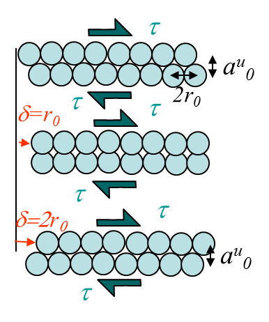
The activation shear stress $\tau$ required for this motion can be evaluated using the model represented in Picture I.32. To do so we will use a sine approximation: from Picture I.32, it appears that the shear stress $\tau$ has to be equal to 0 for slip values $\delta$ equal to 0 and $2r_0$ as both configurations correspond to equilibrium configurations of the crystal, but also for a slip value $\delta=r_0$ for symmetry reasons. Thus $\tau$ is given by:
\begin{equation} \tau = \tau_\text{max}\sin{\frac{\pi\delta}{r_0}} \label{eq:shear} \end{equation}
The shear modulus $G$ is defined as the variation of the shear stress with respect to the variation of shear angle, and can be evaluated from (\ref{eq:shear}):
\begin{equation} G = \left.\frac{d \tau}{d \delta/a_0^u}\right|_{\delta=0} = \tau_\text{max} \frac{\pi a_0^u}{r_0} \label{eq:expG} \end{equation}
If we replace the variables $a_0^u$ and $r_0$ by the values of a BCC crystal we have:
\begin{equation} \tau_\text{max} = \frac{G\sqrt{3}}{4\pi} \label{eq:shearBCC} \end{equation}Using this formula for iron ($G=82$ GPa), one gets $\tau_\text{max}$ of 11 GPa, which is much higher than the measured yield stress, meaning that the shearing mechanism associated to plasticity cannot be a lattice plane motion.
A second possible mechanism is the slip by dislocation glide as illustrated in Picture I.33. This mechanism has as origin the existence of imperfections in a real crystal: substitutional atoms, interstitial atoms or dislocations. A dislocation actually corresponds to missing atoms in the crystal structure as depicted in Picture I.33. Thus the slip can occur by breaking the bonds one by one, leading to a shearing plane mechanism which requires lower activation shear stress.
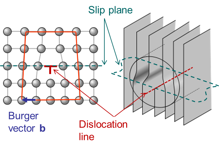
In Picture I.33, as the lattice is purely 2D the only dislocation that propagates is an edge dislocation. To characterize a defect the following material parameters are considered:
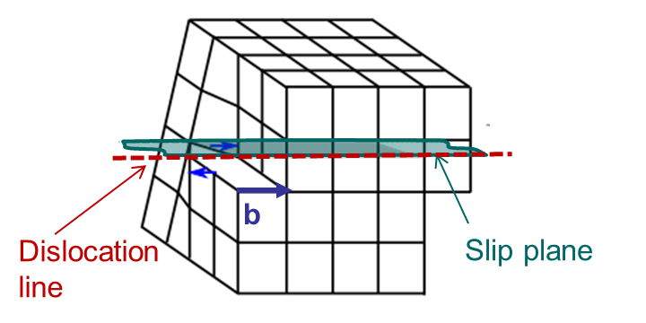
An edge dislocation is characterized by a dislocation line perpendicular to the Burger vector as illustrated in Picture I.34.
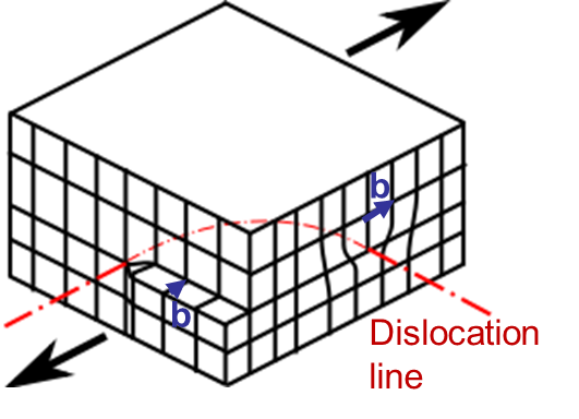
Other kinds of dislocations exist as the screw dislocation for which the burger vector is parallel to the dislocation line, see Picture I.35. A mixed dislocation has a dislocation turning so that it corresponds to an edge dislocation on one side of the crystal and to a screw dislocation on a perpendicular face, see Picture I.36.
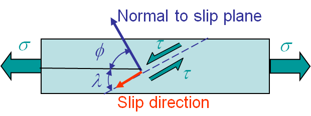
The slip mechanism can be observed experimentally on a single crystal under tension. The plastic deformations will occur along the slip planes as illustrated in Picture I.37. The tension stress $\sigma$ can then be related to the activation stress along the slip plane as $\tau=\sigma\cos\left(\varphi\right)\cos\left(\lambda\right)$. The deformation along the slip plane can be seen in the tension test of a single cadmium crystal in Picture I.38.
The remaining question is "Why do some crystals exhibit plastic deformations, meaning allow for dislocation propagation, contrarily to other ones?" In the following part we will related this behavior the nature of the crystal bonding. Remember that a deformation by dislocations motion corresponds to moving parts of the crystal lattice.
As seen in the previous section, the bonding in a crystal can be ionic, covalent or metallic. We will investigate whether the different bonding allow for dislocation propagation or not. Remember that a dislocation corresponds to an uncompleted atomic plane in the crystal lattice.
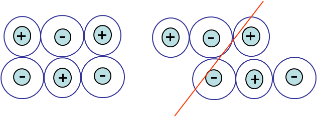
For crystals with ionic bonding the motion of dislocation is difficult. Indeed when moving part of a crystal lattice, there is a configuration for which a positive ion would be in front of another one, see Picture I.39. Thus cleavage requires a lower activation stress than the dislocation propagation, meaning that the ionic crystal is brittle.
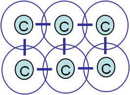
Here again the motion of dislocations is difficult as covalent bonds are strong and directional. As for ionic crystals, cleavage requires a lower activation stress and the crystal is brittle, see Picture I.40.
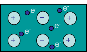
For such crystals, see Picture I.41, the motion of dislocations requires a lower activation stress as bonds are non-directional and result from the negative cloud made of electrons which surrounds the nuclei. So atomic motions along slip directions is possible depending on the crystal structure as it is explained here below.
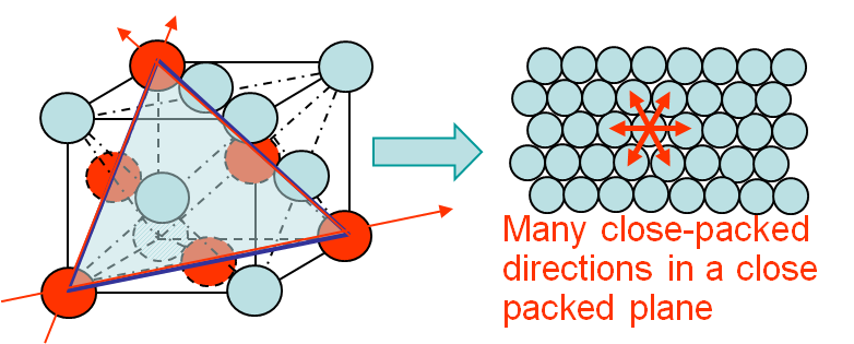
For instance for an FCC crystal as Aluminum or Copper, there exist 4 slip planes. For each slip plane there are 3 slip directions, which make 12 slip systems. Moreover all these slip systems correspond to close-packed planes, see Picture I.42, allowing the motion of dislocations at low energy, and thus at any temperature. These FCC crystals are always ductile.
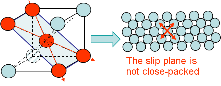
For BCC crystals as ferrite, we have 6 slip planes with 2 slip directions for each slip plane, leading to 12 slip systems as for FCC crystals. However in this case not all the slip systems correspond to close-packed plane, see Picture I.43. This means that at low temperature an atom does not have enough energy to move, and thus the material is brittle as disclocations cannot propagate. On the contrary, at high temperature such a motion is possible (Peierls Stress) and the crystal is ductile. So in the case of a BCC crystal there exists a ductile/brittle transition Temperature (DBTT) below which the material is brittle and above which the crystal is ductile.
Note that it is possible to make the motion of dislocations more difficult by introducing obstacles, leading to harder and less ductile materials. Examples of hardening methods are:
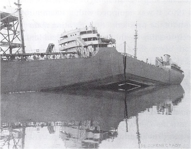
The ships built during WII were made of lower grade steel, leading to a DBTT close to the sea temperature. Failure analyzes were based on a ductile material, meaning that Irwin formula predicts a fracture energy of about $2\gamma_s + W_{pl}$ = 200 kJ/m. In dry docks the ships experienced no problem as the temperature was high enough: existing defects were smaller than the critical size that could be predicted using (\ref{eq:irwin}). However, once the ship was in cold water, below the DBTT, the metal was brittle, with a fracture energy of $2\gamma_s$ = 6800 J/m, and the critical size of a defect was becoming much lower (\ref{eq:griffith}). As consequence some existing defects were larger than the critical size leading to crack propagation, see Picture I.44.
In this section we have focused on the failure of crystals. Other materials are also of interest, and their failure mode is summarized here below.
The failure mode of polymers depends on the structure of the covalent chain structure.
In such a material as Epoxy, the polymers are mainly aligned as shown in Picture I.45 and the molecules are cross-linked by covalent bonding to other ones. Under strain, the material deforms due to bond stretching (as they are already aligned) mechanism. The material thus remains elastic up to a brittle-like failure.
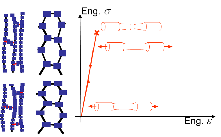
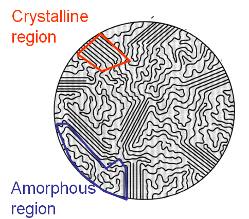
In this case the polymers have some atomic groups, which tend to attract each other and to crystallize into lamellar thin plates: in these regions the chain folds back and forth. The remaining part of the polymer chain has no interaction with other molecules and remains amorphous, see Picture I.46. The behavior of this material strongly depends on the temperature.
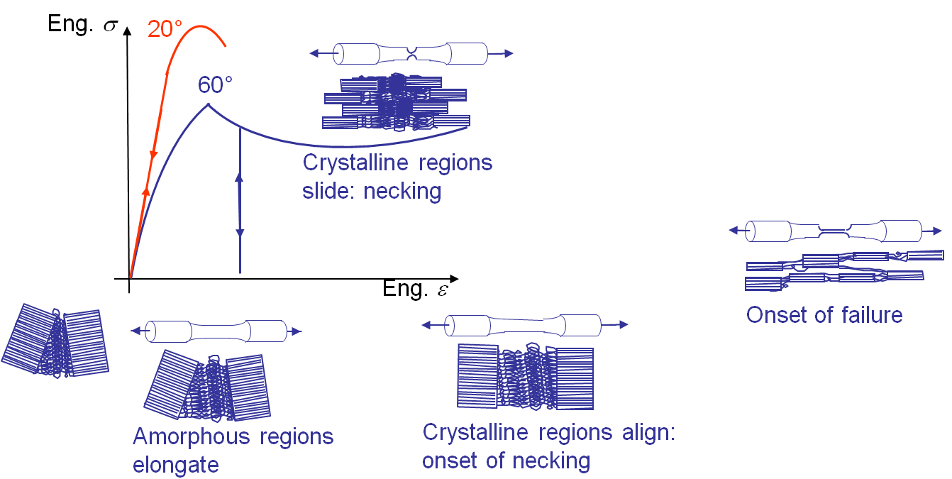
On the one hand, at high temperature the behavior is very different. As long as the stress remains below a certain value, the crystal region remains together and the deformation is due to the disentangling of the long chain molecules. Once the amorphous regions are stretched so that the crystalline regions are aligned, the thermal energy being high enough, the lamellar plates start to slip along one to another leading to irreversible deformation mechanisms corresponding to a necking. Failure occurs as soon as the remaining material volume is small enough to cause the covalent bonding to break. This ductile-like behavior is illustrated in Picture I.47, blue curve.
On the other hand, at low temperature the lamellar plates of the crystalline structure cannot slip and the behavior remains linear elastic until failure, which is brittle-like, see Picture I.47 (red curve).
Examples of such structures are Plexiglas or PVC.
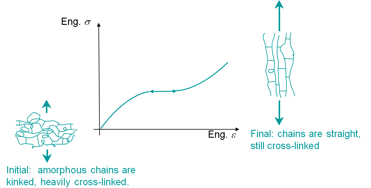
In this case the chains are very long, kinked and heavily cross-linked as in rubber. Such polymers have an amorphous structure, which means that at the microscopic level no real arrangement can be observed. The behavior remains reversible until the brittle-like rupture due to failure of the covalent cross bonds, although elasticity is not linear, Picture I.48.
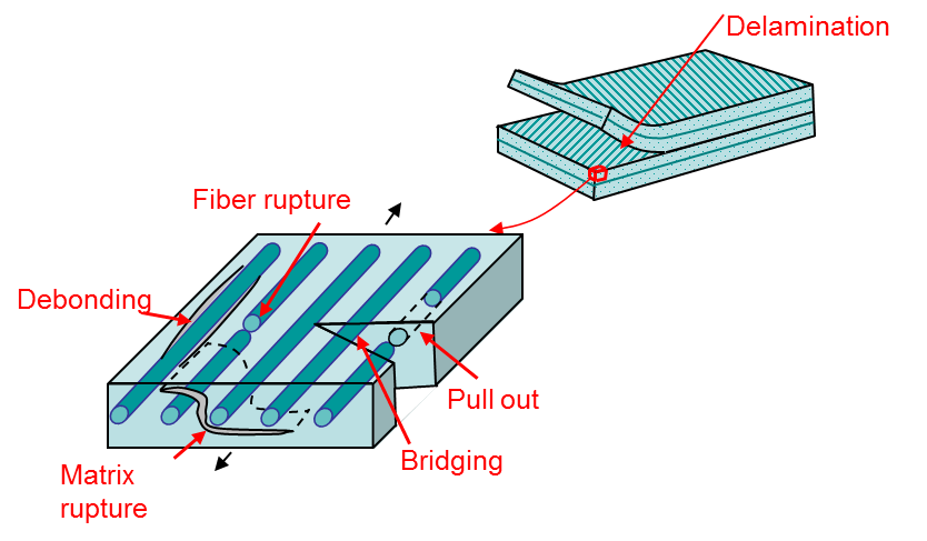
Composites are materials which are heterogeneous at the microscopic level. They are often made of fibers, which can be metals, ceramics, or polymers embedded in a matrix, which can also be made of metals, ceramics, or polymers. For such materials the macroscopic properties depend on the micro-constituents properties and on the fibers arrangement (short fibers, long unidirectional, woven ...).
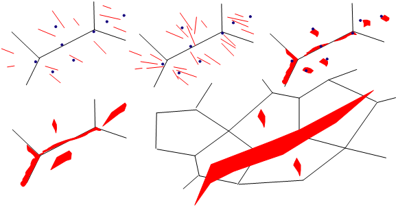
Such materials have very different failures modes that can be explained from the micromechanics, Picture I.49:
At the macroscopic level, the composite materials usually fail as brittle materials.
This section shows that there exist many different failure modes and each one will be modeled in a different way, as will be shown along this class.
![]()