Fracture Mechanics Online Class

Overview > What is fracture mechanics ?

Let us now consider fracture from a physical point of view.

Bonding in materials

There exist mainly 4 different bonding types in materials:

Depending on the nature of the bonding, we will see that the fracture behavior of the material can be different.

Molecular or Van der Waals bonding

Van der Waals bonding (Picture I.9) results from the interaction between dipoles. Examples of materials having such bonds are Argon (Ar), polymers, C₆H₆, graphite. As this kind of bonding is weak, only a reduced amount of energy is necessary to break the bonds.

Ionic bonding

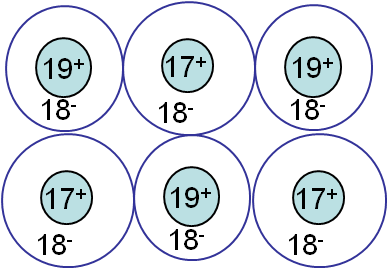
Ionic bonding (Picture I.10) results from the interactions between ions. One or more electrons are transferred from an atom (Cation) to another (Anion), as in NaCl, HCl ... The forces involve in this kind of bonding are non-directional coloumbic forces, reulting in hard & brittle crystals. A material is said to be brittle when it breaks without noticeable plastic deformations.

Covalent bonding

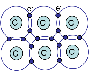
Covalent bonding (Picture I.11) involves bonds between atoms resulting from the "sharing" of electrons, as in CH₄ or diamond. This bonding forces involved are directional and strong, leading to hard & brittle crystals.

Metallic bonding

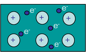
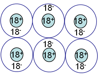
Metallic bonding (Picture I.12) is due to the existence of a cloud or sea of electrons. Theses valence electrons are not shared between two atoms but are common to all the nuclei, and can thus move freely. This leads to materials, such as metals and alloys, which are conductors. This bonding is non-directional and will lead either to brittle or ductile (meaning experiencing plastic deformations before failure) materials as it will be explained.

Free electrons model of a crystal

As previously stated, the nature of the bonding will have an effect on fracture behavior of the material. To model the bonding within the material, we consider the free electrons model. In this model each atom is supposed to have a certain radius r₀, determined by the equilibrium between the attractive and repulsive forces.

The attractive potential

The expression of this potential is different for each kind of bonding but its shape remains similar. For instance for metallic bonding, the attractive potential is due to the interactions between the negative electronic cloud and the positive nuclei, and is given by:

\begin{equation} U_a = - M \frac{z_1 z_2 q^2}{4 \pi \varepsilon_0 r} = -\frac{A_a}{r} \label{eq:attrapot},\end{equation}

where $z_i$ is the valences, $\varepsilon_0$ is the permittivity equal to 8.85 pF/m, $q$ is the electronic charge equal to 1.602*10^-19 C, and $M$ is the Madelungen constant, which depends on the geometric arrangement of the crystal.

The attractive force to which the atoms are submitted is the gradient of the potential (\ref{eq:attrapot}), which is given by:

\begin{equation} f_a = \frac{A_a}{r^2} \label{eq:attra}.\end{equation}

Other examples of such potentials exist as the Lennard-Jones potential which is used to model Van der Waals bonding or the Morse one, which is used for diatomic forces...

The repulsive potential

The repulsive potential is due to the interactions between the electrons within the electronic cloud itself or between the nuclei themselves. It can be expressed as:

\begin{equation} U_r = b\lambda \exp{\frac{-r}{\rho}}= A_r \exp{\frac{-r}{\rho}}, \label{eq:repupot}\end{equation}

where $b$ is the number of adjacent ions, and where both $\lambda$ usually expressed in eV (where eV is an energy unit equal to 1.602*10^-19 J ) and $\rho$ usually expressed in nm are the repulsive parameters. The repulsive force is obtained from the gradient of the potential (\ref{eq:repupot}):

\begin{equation} f_r = -\frac{A_r}{\rho} e^{-\frac{r}{\rho}}. \label{eq:repu}\end{equation}

Total potential

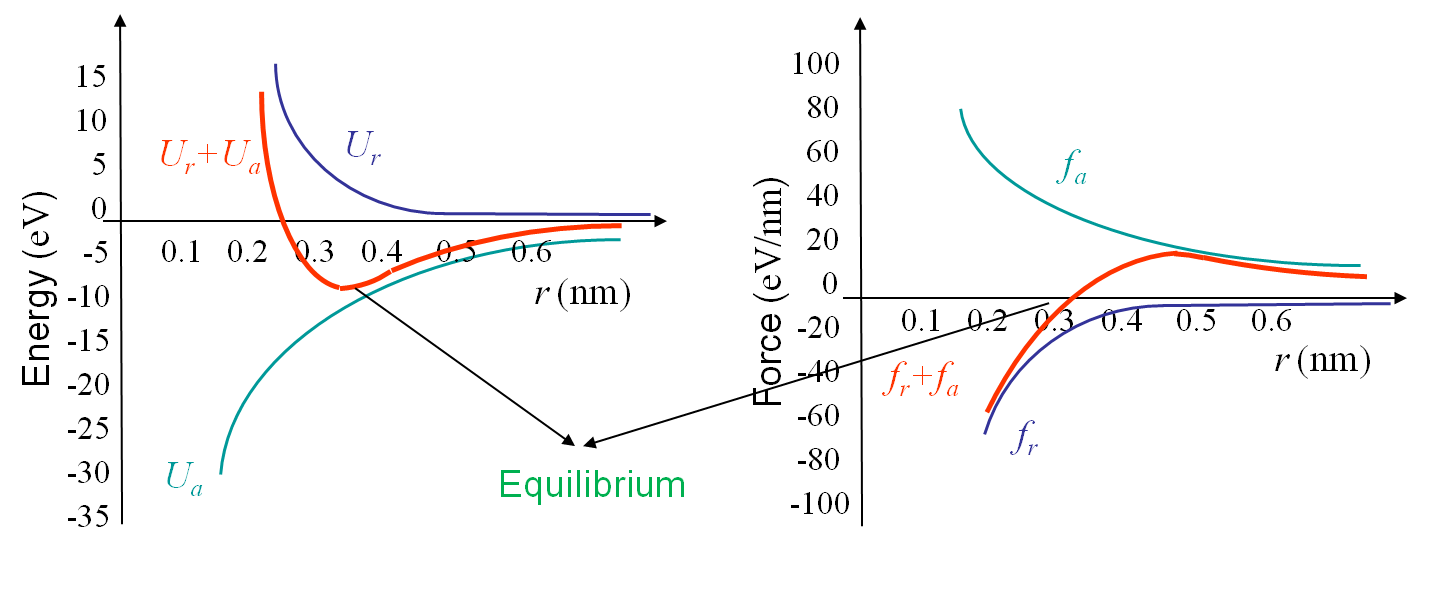
As both potentials have been modeled, it is now possible to determine the equilibrium radius between the spheres. From basic mechanics this equilibrium is obtained for the minimum value of the total potential when the attractive force is equal to the repulsive force as illustrated in Picture I.13 for the ionic bonding in NaCl crystal. If we consider the potentials given by (\ref{eq:attrapot}) and (\ref{eq:repupot}) we find that the equilibrium is obtained for $r_0$ and $U_0$ respectively equal to:

\begin{align} r_0^2\exp{\frac{-r_0}{\rho}} &= \frac{A_a\rho}{A_r}, \text{ and}\\ U_0 &= - \frac{A_a}{r_0}\left[1-\frac{\rho}{r_0}\right]. \label{eq:equpot}\end{align}

Cleavage model of a perfect crystal

The free electrons model can be used to derive the maximal force $f_\text{max}$ that can be reached between the atoms at a corresponding radius $r_\star$, see Pictures I.13. These two values can be evaluated from (\ref{eq:attra}) and (\ref{eq:repu}) and are respectively equal to:

\begin{align} r_\star^3\exp{\frac{-r_\star}{\rho}} &= \frac{2 A_a\rho^2}{A_r},\text{ and}\\ f_\text{max} &= \frac{A_a}{r_\star^2}\left[1-\frac{\rho}{r_\star}\right]. \label{eq:maxforce}\end{align}

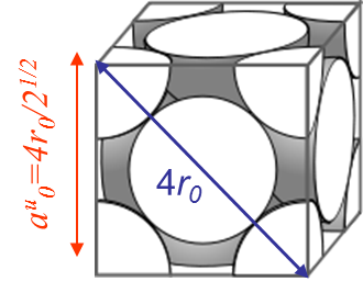
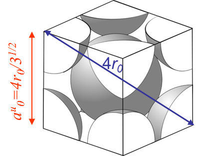
However, the fracture load of a perfect crystal does not only depend on the maximal bonding force between the atoms (\ref{eq:maxforce}), but also depends on the crystal lattice. For instance metallic bonds tend to form crystal structures like in the body-centered crystal (BCC) (iron at low temperature, ferrite ...) or in the face-centered-cubic crystal (FCC) (iron at high temperature, austenite, Aluminum, Copper ...). On Pictures I.14 and I.15 are displayed examples of such lattices, where $r_0$ is the equilibrium radius calculated with the free electron model and where $a_0^u$ is the size of a unit cell.

Once the bonding forces and the lattice structures are known, one has the information needed to evaluate theoretically the failure force along a cleavage plane of a perfect crystal. By definition the stress σ is defined as being the sum of all the forces acting on a surface divided by the surface area:

\begin{equation} \sigma = \frac{1}{S_\text{ref} (\text{plane},r_0)} \sum_i f_i , \label{eq:stress}\end{equation}

where $f_i$ correspond to all the forces between atoms crossing the cleavage plane, see Picture I.16. The young modulus $E$ is by definition obtained from:

\begin{equation} E = \lim_{dr\rightarrow 0}\frac{\sigma\left(r_0+dr\right)-\sigma\left(r_0\right)}{dr}r_0, \label{eq:young}\end{equation}

see Picture I.16. Finally, the surface energy in the case of identical atoms is obtained as follows. Twice the surface energy related to a surface is given by the number of bonds $N_\text{rupture}$ being cut by the cleavage surface times the value of the potential at equilibrium $U_0$ and divided by the reference surface area. This corresponds to the energy one needs to furnish to seperate the upper and lower surfaces (this explains the coefficient 2 in the formula):

\begin{equation} 2\gamma_s = \frac{N_\text{rupture}U_0}{S_\text{ref}}, \label{eq:energsurf}\end{equation}

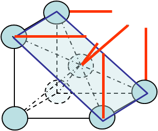
see Picture I.16. Obviously both $S_\text{ref}$ and $N_f$ depend on the crystal lattice as well as on the orientation of the cleavage plane. For instance in the case of cleavage along a (1,1,0) -Miller index- surface of a BCC crystal, see Picture I.17, these values are equal to:

• $S_\text{ref} = \sqrt{2} (a_0^u)^2$
• $N_\text{rupture} = 4 \frac{1}{8}$ (bonds of corner atoms) $+ 2 \frac{1}{8}$ (bonds of the central atom)

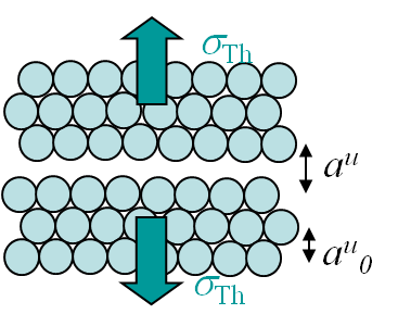
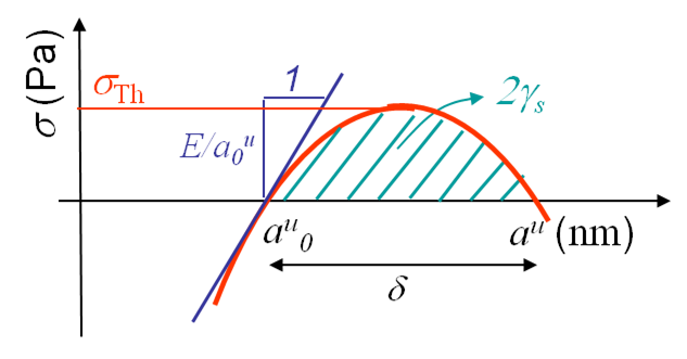
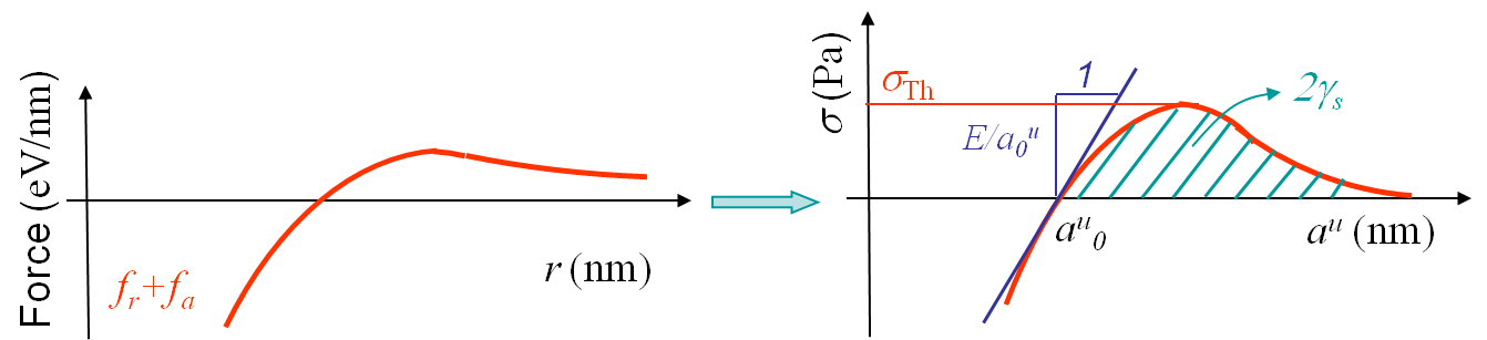
We can now derive a theoretical formula to predict the theoretical value σ_Th (in the case of a brittle perfect crystal) of the tensile strength σ_TS at cleavage. To do so we assume that the atoms on both part of the cleavage plane separate at once as shown in Picture I.18. If we look at the evolution of the bonding force and of the resulting stress in Picture I.16, we see that a sinusoidal approximation can be considered in order of simplifying the calculations, see Picture I.19:

\begin{equation} \sigma = \sigma_{\text{Th}} \sin{\left(\pi\frac{a^u-a^u_0}{\delta}\right)}. \label{eq:stresssinapprox} \end{equation}

The missing parameter $\delta$ can be obtained in terms of the Young modulus by using (\ref{eq:young}):

\begin{equation} \frac{E}{a^u_0} = \left.\frac{d\sigma}{d a^u}\right|_{a_0^u} = \sigma_{\text{Th}} \frac{\pi}{\delta}. \label{eq:expyoung} \end{equation}

Finally (twice) the surface energy can be introduced by using its definition -the work of separation- which corresponds to the integral of the stress tensor (\ref{eq:stresssinapprox}) from the equilibrium distance to the value for which the stress tensor vanishes:

\begin{equation} 2\gamma_s = \int_{a_0^u}^{a_0^u+\delta} \sigma da^u = 2 \sigma_{\text{Th}}\frac{\delta}{\pi}. \label{eq:expenergsurf} \end{equation}

Combining (\ref{eq:expyoung}) and (\ref{eq:expenergsurf}) leads to the theoretical tensile strength $\sigma_\text{Th}$:

\begin{equation} \sigma_{\text{Th}} = \sqrt{\frac{E\gamma_s}{a^u_0}}. \label{eq:tensstress} \end{equation}

The table below shows some examples of the theoretical tensile strength computed using (\ref{eq:tensstress}):

Table I.1: Theoretical strength.

	$a^u_0$ [nm]	$E$ [GPa]	$\gamma_s$ [J m^{-2}]	$\sigma_\text{Th}$ [GPa]
Glass	0.3	60	21	64 !!!
Steel (low T)	0.3	210	3400	1,500 !!!

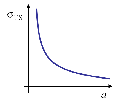
When comparing the values of the theoretical model in Table I.1 to the values obtained from experiments, it appears that they are some orders of magnitudes too high. This discrepancy was explained by Griffith in 1920 when he analysed the influence of a scratch of size $2a$ on a glass plate - thermally threated to remove the residual stresses- on the tensile strength. He observed a dependency which follows the equation:

\begin{equation}\sigma_{\text{TS}}\sqrt{a} \div \sqrt{E\, 2\gamma_s}, \label{eq:griffith} \end{equation}

as illustrated on Picture I.20. The experiments of Griffith put in evidence the effect of a defect as a scratch (which is actually a crack) on the material strength. Fracture mechanics was pioneered: the resistance of a structure could only be evaluated by considering its defects.

Ludovic Noels, E-mail: L.Noels @ ulg.ac.be • University of Liège • Computational & Multiscale Mechanics of Materials (CM3)