SIF Computation > Analytical methods (LEFM)
Methodology: Westergaard approach
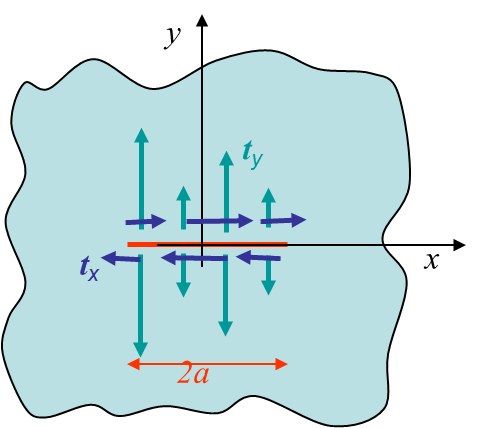
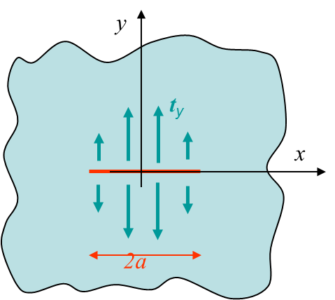
We can now compute the analytical solution for an infinite plane with a centered crack. At first we consider the problem of crack surfaces loaded as shown in Picture IV.1. For a pure mode I loading we consider the particular loading case shown in Picture IV.2: $\mathbf{t}=t_y\mathbf{e}_2$ with $t_y(-x)=t_y(x)$, $t_y(-y)=-t_y(y)$ . For such a loading we know that the shear stress should vanish along the $x$ axis: $\mathbf{\sigma}_{xy}=0$ for $y=0$. Using the expression of the stress field one has
\begin{equation} \mathbf{\sigma}_{xy} = i \frac{\zeta\bar{\Omega}''+\bar{\omega}''-\bar{\zeta}\Omega''-\omega''}{2} =0\;\;\text{ if } y=0. \label{eq:shearStressModeI} \end{equation}
The solution to this problem is to select $\omega''=-\zeta\Omega''$ as this leads directly to
\begin{equation}\left\{\begin{array}{r c l} \mathbf{\sigma}_{xy} &=& -y2\mathcal{R}\left(\Omega''\right)\\ \omega' &=& - \zeta\Omega' + \Omega + C \end{array}\right.\,.\label{eq:omegaprimModeI}\end{equation}
The first line of equation (\ref{eq:omegaprimModeI}) demonstrates that $\mathbf{\sigma}_{xy}=0$ for $y=0$. The second line, which is the integration of $\omega''=-\zeta\Omega''$ with $C$ a constant, allows the complete stress and displacement fields, which were found to be
\begin{equation} \left\{ \begin{array}{r c l} \mathbf{\sigma}_{xx} &= &\Omega'+\bar{\Omega}' - \frac{\bar{\zeta}\Omega''+\omega''+ \zeta\bar{\Omega}''+ \bar{\omega}''}{2}\\ \mathbf{\sigma}_{yy} &=&\Omega'+\bar{\Omega}' + \frac{\bar{\zeta}\Omega''+\omega''+ \zeta\bar{\Omega}''+ \bar{\omega}''}{2}\\ \mathbf{\sigma}_{xy} &=& i \frac{\zeta\bar{\Omega}''+\bar{\omega}''-\bar{\zeta}\Omega''-\omega''}{2}\\ \mathbf{u} &=& -\frac{1+\nu}{E}\left(\zeta\bar{\Omega}'+\bar{\omega}' + \kappa \left(\zeta\right)\right) \end{array} \right.\,, \end{equation}
\begin{equation} \left\{ \begin{array}{r c l} \mathbf{\sigma}_{xx} &=& 2\mathcal{R}\left(\Omega'\right)-2 y\mathcal{I}\left(\Omega''\right)\\ \mathbf{\sigma}_{yy} &=& 2\mathcal{R}\left(\Omega'\right)+2 y\mathcal{I}\left(\Omega''\right)\\ \mathbf{\sigma}_{xy} &=& -y2\mathcal{R}\left(\Omega''\right)\\ \mathbf{u}_x &=& \mathcal{R}\left(\mathbf{u}\right) = \frac{1+\nu}{E}\left[\left(\kappa-1\right)\mathcal{R}\left(\Omega\right)-2y\mathcal{I}\left(\Omega'\right)-\mathcal{R}\left(C\right)\right]\\ \mathbf{u}_y &=& \mathcal{I}\left(\mathbf{u}\right) = \frac{1+\nu}{E}\left[\left(\kappa+1\right)\mathcal{I}\left(\Omega\right)-2y\mathcal{R}\left(\Omega'\right)+\mathcal{I}\left(C\right)\right] \end{array} \right.\label{equa1}\,.\end{equation}
At this level only $\Omega$ has to be defined so that the stress and displacement fields satisfy the boundary conditions shown in Picture IV.2. Assuming a constant value for $t_y$ the solution $\Omega\left(x \geq 0\right)$ reads
\begin{equation} \Omega' \left(x \geq 0\right)= \frac{t_y}{2}\left(\frac{ \zeta}{\sqrt{\zeta^2-a^2}}-1\right) \Longrightarrow \left\{\begin{array}{r c l} \Omega'' = - \frac{t_y}{2}\left(\frac{ a^2}{\sqrt{\zeta^2-a^2}^3}\right)\\ \Omega = \frac{t_y}{2}\left(\sqrt{\zeta^2-a^2}-\zeta+C_1\right) \end{array}\right. \,.\label{equa2}\end{equation}
In the context of this class we will not establish this last relation, but instead show that it satisfies the boundary conditions of the problem
Remark: The general solution (Sedov, 1972) reads
\begin{equation}\Omega' = \frac{1}{2\pi\sqrt{\zeta^2-a^2}}\int_{-a}^{a} t_y\left(\xi\right) \frac{\sqrt{a^2-\xi^2}}{\zeta-\xi} d\xi \,.\end{equation}
Verification of the solution
We need to check if the above solution (\ref{equa2}) is compatible with the boundary conditions of Picture IV.2.
Displacement field
The first thing to check is to verify the symmetry with respect to the Ox-axis. First we notice that if $\mathcal{I}\left(C_I\right)=0$ one has
\begin{equation} \left.\begin{array}{r c l} \Omega\left(\bar{\zeta}\right) &= &\bar{\Omega}\\ \Omega'\left(\bar{\zeta}\right)& = &\bar{\Omega'} \end{array}\right\}\Longrightarrow \left\{\begin{array}{r c l } \mathcal{R}\left(\Omega\left(x-i y\right)\right) &=&\mathcal{R}\left(\Omega\left(x+ i y\right)\right)\\ \mathcal{R}\left(\Omega'\left(x-i y\right)\right) &=&\mathcal{R}\left(\Omega'\left(x+ i y\right)\right)\\ \mathcal{I}\left(\Omega\left(x-i y\right)\right) &=&-\mathcal{I}\left(\Omega\left(x+ i y\right)\right)\\ \mathcal{I}\left(\Omega\left(x-i y\right)\right) &=&-\mathcal{I}\left(\Omega\left(x+ i y\right)\right)\end{array}\right. .\label{eq:conjugatedOmega} \end{equation}
Using these results in (\ref{equa1}) directly leads to
\begin{equation} \mathbf{u}_x(-y) = \mathbf{u}_x(y), \quad \mathbf{u}_y(-y) = \mathbf{u}_y(y),\end{equation}
if $\mathcal{I}\left(C\right)=0$.
Stress field
One condition that needs to be satisfy is to obtain a vanishing far away field, see Picture IV.2: $\mathbf{\sigma}_{xx}\rightarrow\ 0$ , $\mathbf{\sigma}_{yy} \rightarrow\ 0$, and $\mathbf{\sigma}_{xy} \rightarrow\ 0$ at infinity. The stress field depends only on $\mathcal{R}\left(\Omega'\right)$ and on $y\mathcal{I}\left(\Omega''\right)$ as shown by equation (\ref{equa1}). So this boundary condition is equivalent to
\begin{equation}\left\{\begin{array}{ l c r} \lim_{|\zeta|\rightarrow\infty} \mathcal{R}\left(\Omega'\right)& =& 0\\ \lim_{|\zeta|\rightarrow\infty} y \mathcal{I}\left(\Omega''\right) &=&0 \end{array}\right.\,,\end{equation}
which is the case as it can be seen from equation (\ref{equa2}). We thus have:
\begin{equation}\mathbf{\sigma}_{xx}(\zeta\rightarrow\infty)\rightarrow0, \quad \mathbf{\sigma}_{yy} (\zeta\rightarrow\infty) \rightarrow 0 ,\text{ and } \mathbf{\sigma}_{xy} (\zeta\rightarrow\infty) \rightarrow 0 .\end{equation}
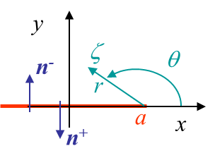
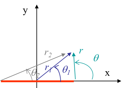
The other boundary condition is the loading $t_y$ on the crack lips, $\zeta = x\pm i|\epsilon|$, $\epsilon \rightarrow 0$, $|x|< a$, which should be recovered from the stress field. To analyze this condition we consider the polar coordinates linked to the crack tip, see Picture IV.3. The square root that appears in equation (\ref{equa2}) can be expressed as
\begin{equation} \sqrt{\zeta-a}=\sqrt{r \exp{\left(i\theta\right)}} = \sqrt{r}\cos{\frac{\theta}{2}}+i\sqrt{r}\sin{\frac{\theta}{2}}. \end{equation}
This expression can be evaluated on the crack lips $\zeta = x\pm i|\epsilon|$, $\epsilon \rightarrow 0$, $|x|< a$ by considering $\theta\rightarrow\pm\pi$, leading to
\begin{equation} \lim_{\theta\rightarrow\pm\pi}\sqrt{\zeta-a}=\pm i\sqrt{r}=\pm i \sqrt{(a-x)}. \end{equation}
Thus using equation (\ref{equa2}) one has
\begin{equation} \lim_{\theta\rightarrow\pm\pi} \Omega' = \pm \frac{t_y}{2}\frac{x}{i \sqrt{a+x} \sqrt{a-x}} -\frac{t_y}{2} = \mp\frac{i x t_y}{2 \sqrt{a^2-x^2}} - \frac{t_y}{2} \end{equation}
The stress field on the crack lips can then be evaluated from (\ref{equa1}) as being $\mathbf{\sigma}_{yy}=2\mathcal{R}(\Omega')$, and the crack lips loading follows from $\mathbf{t}=\mathbf{n} \cdot \mathbf{\sigma}$. The direction of the normal to the crack lips can be seen in Picture IV.3 and one can directly get $\mathbf{t}= \mp 2\mathcal{R}(\Omega') \mathbf{e}_2= \pm t_y \mathbf{e}_2$, which satisfies the boundary condition on the crack lips.
Symmetry with respect to Oy
The last condition to verify is the symmetry and continuity of the solution along the Oy-axis. To this end we evaluate the solution (\ref{equa1}) for $x=0$, which yields
\begin{equation} \left\{\begin{array}{l c l} \Omega''\left(x=0\right) &= &\frac{t_y}{2}\left(\pm\frac{ia^2}{\sqrt{y^2+a^2}^3}\right)\,;\\ \Omega'\left(x=0\right) &=& \frac{t_y}{2}\left(\pm\frac{y}{\sqrt{y^2+a^2}}-1\right)\\ \Omega\left(x=0\right) &=& \frac{t_y}{2}\left(\pm i \sqrt{y^2+a^2}-i y-C_1\right) \,.\end{array}\right. \label{equ_omega} \end{equation}
Using (\ref{equa2}), we can directly conclude that in order to satisfy $u_x(x=0)=0$ we need $\mathcal{R}(C)=0$, and in order to have $\sigma_{xy}(x=0)=0$ we need $\mathcal{R}(C_1)=0$. As the imaginary part of the integration constants were also found to be zero, we thus have $C=C_1=0$.
Solution for the mode I crack lips loading case
As the solution (\ref{equa1}) with $C=C_1=0$ has been found to satisfy the boundary conditions, we can use it in (\ref{equa2}) in order to evaluate the complete solution, first on the crack lips and then ahead of the crack tip.
Crack Opening Displacement COD
The field of interest is the opening of the crack resulting from the crack lips loading. Equation (\ref{equa1}) with $C=C_1=0$ allows evaluating the displacement field from (\ref{equa2}), which reduces into
\begin{equation} \left\{\begin{array}{r c l} \Omega &=& \frac{t_y}{2}\left(\sqrt{\zeta^2-a^2}-\zeta\right)\,;\\ u_y &=&\mathcal{I}\left(u\right) = \frac{1+\nu}{E}\left[\left(\kappa+1\right)\mathcal{I}\left(\Omega\right)-2y\mathcal{R}\left(\Omega'\right)\right]\,.\end{array}\right. \label{eq:uCrack} \end{equation}
Proceeding as before to evaluate the field on the crack lips $\zeta = a-r\pm i|\epsilon|$, $\epsilon \rightarrow 0$, one has
\begin{equation}\left\{ \begin{array}{l} \sqrt{\zeta-a}=\sqrt{r \exp{\left(i\theta\right)}}= \sqrt{r}\cos{\frac{\theta}{2}}+i\sqrt{r}\sin{ \frac{\theta}{2}}\,;\\ \Longrightarrow \lim_{\theta\rightarrow\pm\pi}\sqrt{\zeta-a}=\pm i\sqrt{r}=\pm i \sqrt{(a-x)} \,;\\ \Longrightarrow \lim_{\theta\rightarrow\pm\pi} \Omega = \frac{t_y}{2}\left(\pm i \sqrt{ a^2-x^2} -x \right)\,. \end{array}\right. \end{equation}
This allows evaluating the displacement (\ref{eq:uCrack}) on the crack lips as
\begin{equation} \lim_{\theta\rightarrow\pm\pi} u_y =\pm \frac{\left(1+\nu\right)\left(\kappa+1\right)t_y} {2E} \sqrt{a^2-x^2}\,. \end{equation}
This last equation leads to the expression of the crack opening displacement (COD), which is the opening between the two lips of the crack:
\begin{equation} \left[\!\left[ u_y\right]\!\right] = \frac{\left(1+\nu\right)\left(\kappa+1\right)t_y} {E} \sqrt{a^2-x^2} \,.\label{eq:COD}\end{equation}
Stress field ahead of the crack tip
Ahead of the crack tip we are interested in the stress field in order to evaluate the SIF. For $\zeta = a-r\pm i|\epsilon|$, $\epsilon \rightarrow 0$, we can simplify the equation (\ref{equa2}) into:
\begin{equation} \left\{\begin{array}{l c l} \Omega\left(\theta=0\right)&=&\frac{t_y}{2}\left(\sqrt{x^2-a^2}-x+C_1\right) \rightarrow \frac{t_y}{2}\left(\sqrt{2ar}-a+C_1\right)\,;\\ \Omega'\left(\theta=0\right) &=& \frac{t_y}{2}\left(\frac{x}{\sqrt{x^2-a^2}}-1\right)\rightarrow \frac{t_y}{2}\left(\sqrt{\frac{a}{2r}}-1\right)\,;\\ \Omega''\left(\theta=0\right)&= &- \frac{t_y}{2}\left(\frac{ a^2}{\sqrt{x^2-a^2}^3}\right)\rightarrow - \frac{t_y}{4r}\sqrt{\frac{a}{2r}}\,, \end{array}\right. \end{equation}
where we have also developed the assymptotic field using $r\rightarrow 0^+$. We can now use that $\Omega$ function to evaluate the stress field (\ref{equa1}) ahead of crack tip as
\begin{equation} \mathbf{\sigma}_{xx}\left(\theta=0\right) = \mathbf{\sigma}_{yy}\left(\theta=0\right)= 2 \mathcal{R}\left(\Omega'\right) = t_y \left(\frac{x}{\sqrt{x^2-a^2}}-1\right)\rightarrow t_y \left(\sqrt{\frac{a}{2r}}-1\right)\,; \label{eq:SIFCase1}\end{equation} \begin{equation} \mathbf{\sigma}_{xy}\left(\theta=0\right) = 0\,. \end{equation}
However this expression holds for the crack lips loading as shown in Picture IV.2, which is not the case of a usual crack problem in Mode I.
Crack in an infinite plate
Mode I: Opening
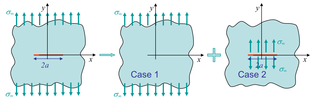
In the previous section we have solved the problem of an infinite plate with a loading applied on the crack lips, see third figure of Picture IV.4. The problem of interest is actually the mode I crack loading as shown in the first figure of Picture IV.4. As we are in linear elasticity, we can apply the supperposition principle to the following two cases:
- Case 1: uniform tension;
- Case 2: solved here above with $t_y = \sigma_\infty$.
\begin{equation} \left. \begin{array}{l c l} \mathbf{\sigma}_{yy}&=&\mathbf{\sigma}_\infty\\ \mathbf{\sigma}_{xx}&=&\mathbf{\sigma}_{xy}=0\end{array}\right\}\Longrightarrow\left\{ \begin{array}{ r c l} \epsilon_{xx}& = &\frac{\left(1+\nu\right)\left(3-\kappa\right)}{4E}\mathbf{\sigma}_\infty\,;\\ \epsilon_{yy}& =& \frac{\left(1+\nu\right)\left(1+\kappa\right)}{4E}\mathbf{\sigma}_\infty\,;\\ \epsilon_{xy}& =& 0\,;\\ u_{x} &=&\frac{\left(1+\nu\right)\left(3-\kappa\right)}{4E}\mathbf{\sigma}_\infty x\,;\\ u_{y} &=&\frac{\left(1+\nu\right)\left(1+\kappa\right)}{4E}\mathbf{\sigma}_\infty y\,.\\ \end{array}\right. \label{eq:SIFcase2} \end{equation}
The solution of the problem is thus obtained by the superposition of the full stress fields (\ref{eq:SIFCase1}) and (\ref{eq:SIFcase2}). The stress field ahead of the crack tip is obtained, at $y=0$, for $x>a$ and reads
\begin{equation} \mathbf{\sigma}_{yy} = \mathbf{\sigma}^{\text{case I}}_{yy} + \mathbf{\sigma}^{\text{case II}}_{yy} = \mathbf{\sigma}_\infty \frac{x}{\sqrt{x^2-a^2}} \rightarrow \mathbf{\sigma}_\infty \sqrt{\frac{a}{2r}}\,,\label{eq:SIFsup1} \end{equation}
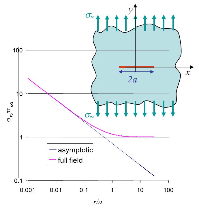
where the asymptotic field has also been computed. The comparison between the full field and the asymptotic solution is illustrated in Picture IV.5. The stress intensity factor is directly obtained from
\begin{equation} K_I = \lim_{r\rightarrow 0} \left(\sqrt{2\pi r}\left.\mathbf{\sigma}_{yy}^{\text{mode I}}\right|_{\theta=0} \right) = \mathbf{\sigma}_\infty \sqrt{ a \pi}\label{eq:SIFIsup}\,.\end{equation}
As expected the stress intensity factor is linear with the applied loading as we are in linear elasticity. It also depends on the square root of the crack size.
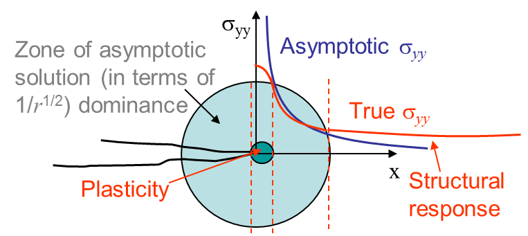
In Picture IV.5 it can be seen that the asymptotic solution is only valid near the crack tip when compared to the exact stress field. Moreover it can be seen that both solutions are singular at the crack tip, which is not physical. This means that the asymptotic solution is only valid within a ring centered at the crack tip as illustrated in Picture IV.6.
Mode II: Sliding
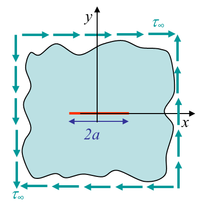
For a crack loaded in mode II, see Picture IV.7, the same method can be applied. In brief one would find:
- For mode II loading: $\sigma_{yy} = 0$ for $y=0$ so the Westergaard function reads \begin{equation}\omega'' = -2 \Omega' - \zeta \Omega''\,.\end{equation}
- For the crack lips subjected to a tangential loading $t_x$, the remaining function is selected to be \begin{equation} \Omega' = \frac{-i}{2\pi\sqrt{\zeta^2-a^2}}\int_{-a}^{a} t_x\left(\xi\right) \frac{\sqrt{a^2-\xi^2}}{\zeta-\xi} d\xi \,.\end{equation}
- Applying the superposition principle with a uniform shearing $\tau_\infty$ and considering $t_x=\tau_\infty$ lead to \begin{equation} K_{II} = \lim_{r\rightarrow 0} \left(\sqrt{2\pi r}\left.\mathbf{\sigma}_{xy}^{\text{mode II}}\right|_{\theta=0} \right) = \tau_\infty \sqrt{ a \pi} \label{eq:SIFIIsup}\,. \end{equation}
Mode III: Shearing
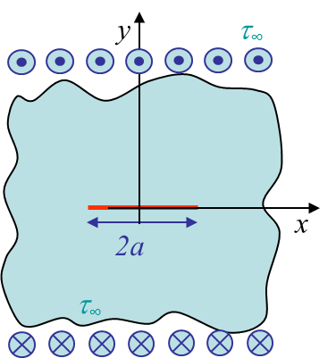
The problem of the crack loaded in Mode III is illustrated in Picture IV.8. Using the definition of the strain tensor and applying the Hooke's law lead to the expression of the stress field in terms of the displacement field:
\begin{equation} \left\{\begin{array}{r c l} \mathbf{\varepsilon}_{\alpha z}&=&\frac{1}{2}\mathbf{u}_{e,\alpha}\,;\\\Rightarrow \sigma_{\alpha z} &=&\frac{E}{1+\nu}\mathbf{\varepsilon}_{\alpha z}=\frac{E}{2(1+\nu)}\mathbf{u}_{z,\alpha}\,.\end{array}\right. \end{equation}
We can now apply the linear momentum conservation law $\mathbf{\nabla}\cdot\mathbf{\sigma}$ to this expression to find
\begin{equation} \sigma_{\alpha z, \alpha} = 0 \Rightarrow \nabla^2 \mathbf{u}_z=0 \label{eq:sigIIItmp} \,.\end{equation}
From this last result, using Cauchy-Riemann relations, we can deduce that $\mathbf{u}_z$ is the imaginary part of a function $z(\zeta)$. As the Cauchy-Riemann relation implies
\begin{equation} \partial_\zeta z = \partial_x z = - i \partial_y z \,, \end{equation}
equation (\ref{eq:sigIIItmp}) leads to
\begin{equation}\begin{cases} \sigma_{yz} = \frac{E}{2\left(1+\nu\right)}u_{z,y} = \frac{E}{2\left(1+\nu\right)}\partial_y\mathcal{I}\left(z\right) = \frac{E}{2\left(1+\nu\right)} \mathcal{I}\left(i z'\right) \,;\\ \sigma_{xz} = \frac{E}{2\left(1+\nu\right)}u_{z,x} = \frac{E}{2\left(1+\nu\right)}\partial_x\mathcal{I}\left(z\right) = \frac{E}{2\left(1+\nu\right)} \mathcal{I}\left(z'\right)\,.\end{cases} \label{eq:sigIIIcomp}\end{equation}
The function $z(\zeta)$ has to be chosen so that it satisfies the boundary conditions of the problem illustrated in Picture IV.7. The solution of the problem reads
\begin{equation} z\left(\zeta\right) = \frac{2 \tau_{\infty}\left(1+\nu\right)}{E}\sqrt{\zeta^2-a^2} \end{equation}
as it leads to
\begin{equation} \left\{\begin{array}{r c l} \sigma_{yz} &= &\frac{E}{2\left(1+\nu\right)} \mathcal{I}\left(i z'\right) \Longrightarrow \tau_\infty\mathcal{R}\left(\frac{\zeta}{\sqrt{\zeta^2-a^2}}\right)\,;\\ \mathbf{u}_z&=&I(z)\,.\end{array}\right. \label{eq:sigIII} \end{equation}
Indeed this solution satisfies the boundary conditions as
- The symmetry is satisfied: $z(\bar{\zeta})= \bar{z}\Longrightarrow \mathbf{u}_z(-y)=-\mathbf{u}_z(-y)$;
- The far away field is satisfied as $\sigma_{xy}\rightarrow \pm \tau_{\infty}$ for $y\rightarrow \pm\infty$;
- The crack lips are also stress free.
This last point can be demonstrated as follows.
Considering the angles defined on Picture IV.9, one can evaluate the following functions on the crack lips.
\begin{equation}\left\{\begin{array}{l} \lim_{\theta \rightarrow \pm \pi} \zeta = x\,;\\ \lim_{\theta \rightarrow \pm \pi} \sqrt{\zeta-a} = \lim_{\theta \rightarrow \pm \pi} \sqrt{r}\exp{\left(i\frac{\theta}{2}\right)} = \pm i \sqrt{a-x}\,; \\ \lim_{\theta_2 \rightarrow 0^\pm} \sqrt{\zeta+a} = \lim_{\theta_2 \rightarrow 0^\pm} \sqrt{r_2}\exp{\left(i\frac{\theta_2}{2}\right)} = \sqrt{x+a} \end{array}\,.\right. \end{equation}
Thus the stress field (\ref{eq:sigIII}) on the crack lips is found to be
\begin{equation} \lim_{\theta \rightarrow \pm \pi,\, \theta_2\rightarrow 0} \sigma_{yz} = \lim_{\theta \rightarrow \pm \pi,\, \theta_2\rightarrow 0}\tau_\infty \mathcal{R}\left(\frac{\zeta}{\sqrt{\zeta^2-a^2}}\right) \rightarrow \tau_\infty \mathcal{R}\left(\frac{\mp i x}{\sqrt{a^2-x^2}}\right) = 0 \,,\end{equation}
which satsifies the stress free condition on the crack. The stress field (\ref{eq:sigIII}) is thus the solution of the mode III problem. Ahead of the crack tip ($y=0$ and $x =a+r$), this solution reads
\begin{equation} \mathbf{\sigma}_{yz} = \tau_\infty \mathcal{R}\left(\frac{a+r}{\sqrt{r^2+2ar}}\right) \rightarrow \tau_\infty\sqrt{\frac{a}{2r}}\,, \end{equation}
where we have expressed the assymptotic field. The stress intensity factor can thus be directly evaluated from
\begin{equation} K_{III} = \lim_{r\rightarrow 0} \left(\sqrt{2\pi r}\left.\mathbf{\sigma}_{yz}^{\text{mode III}}\right|_{\theta=0} \right) = \tau_\infty\sqrt{\pi a} \,.\label{eq:SIFIII} \end{equation}
As it has been shown, some analytical solutions exist for simple geometries, but they lack of generalities. This has motivated the development of numerical and semi-analytical methods in order to be able to compute the SIFs for more general cases.
A semi analytical method: the boundary collocation method
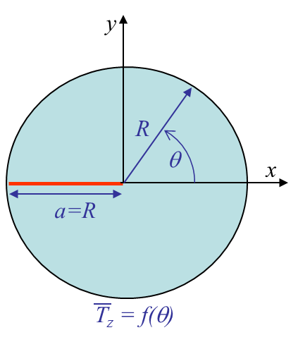
One of the most popular semi-analytical method is the boudnary collocation one. To give an idea on how it can be applied we consider a crack in a finite circular plate under mode III loading, see Picture IV.10. From the general out of plane solution (\ref{eq:sigIIIcomp}), one can define the complex stress
\begin{equation} \tau = \sigma_{yz} + i \sigma_{xz} = \frac{E}{2\left(1+\nu\right)}z'\,.\end{equation}
Defining a complex outward normal $\mathbf{n} = \mathbf{n}_x + i \mathbf{n}_y$ allows thus to compute the boundary force as
\begin{equation} \bar{\mathbf{T}}_z = \sigma_{xz} \mathbf{n}_x + \sigma_{yz} \mathbf{n}_y =\mathcal{I}\left(\tau \mathbf{n}\right) \,.\label{eq:Tz}\end{equation}
The solution of the problem is given from the complex function $z(\zeta)$. To find its expression we use the Laurent series $\tau\left(\zeta\right) = \sum_{n=-\infty}^\infty a_n \left(\zeta-\zeta_0\right)^{n}$ with $a_n =\frac{1}{2 i \pi}\int_{\mathcal{C}} \frac{z\left(\xi\right)}{\left(\xi-\zeta_0\right)^{n+1}}d\xi$ the unknown coefficients. However, for our problem with a crack in $\theta=\pm \pi$, we instead use
\begin{equation}\tau\left(\zeta\right) = \sum_{n=-\infty}^\infty a_n \zeta^{n-\frac{1}{2}} \,.\end{equation}
Indeed in this case we directly have
\begin{equation} \lim_{\theta\rightarrow\pi}\sigma_{yz} = \lim_{\theta\rightarrow\pi}\mathcal{R} \left(\tau\right) = \lim_{\theta\rightarrow\pi} \sum_{n=-\infty}^\infty a_n r^{n-\frac{1}{2}} \cos{\left(\frac{2n-1}{2} \pi\right)} = 0 \,,\end{equation}
which satisfies the boudary condition on the crack lips. Moreover as we have a finite displacement we restrain $n$ to $n=0, 1, 2, ...$. Finally we have the solution of our problem as
\begin{equation}\tau\left(\zeta\right) = \sum_{n=0}^\infty a_n \zeta^{n-\frac{1}{2}}\label{eq:tauzeta}\,,\end{equation}
with the SIF given by
\begin{equation} K_{III} = \lim_{r\rightarrow 0} \left(\sqrt{2\pi r}\left.\sigma_{yz}\right|_{\theta=0} \right) = \sqrt{2\pi} a_0\,. \end{equation}
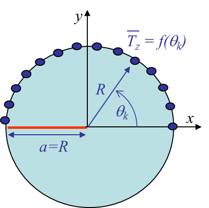
To solve this problem we now need to find the unknows $a_n$, which are obtained by defining $m$ collocation points on the boundary of the domain, see Picture IV.11. At these points we can evaluate (\ref{eq:Tz}) as
\begin{equation} \bar{\mathbf{T}}_z\left(\theta_k\right) =\mathcal{I}\left(\tau\left(\theta_k\right) \mathbf{n}\left(\theta_k\right)\right)\,.\end{equation}
Using (\ref{eq:tauzeta}), this last result becomes
\begin{equation} \bar{\mathbf{T}}_z\left(\theta_k\right) = \mathcal{I}\left(\sum_{n=0}^p a_n r_k^{n-\frac{1}{2}}\exp{\left(i\frac{2n-1}{2}\theta_k\right)} \mathbf{n}\left(\theta_k\right)\right)\,,\label{eq:colloc} \end{equation}
for $k = 1, ..., m$. As $ \bar{\mathbf{T}}_z\left(\theta_k\right)$ is known from the problem statement, if we limit the series to the order $p$ with $p+1\leq m$, we can solve the system of $m$ equations with $p+1$ unknowns.
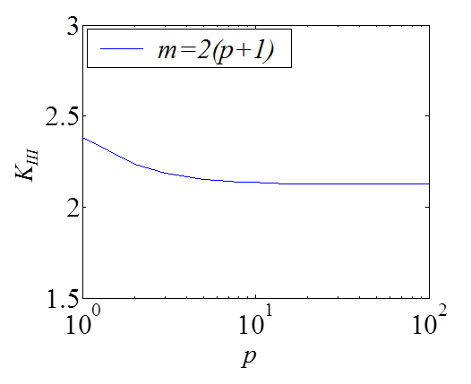
As an example we can consider $R=1$ and the boundary condition to be $\bar{\mathbf{T}}_z = \sin{\theta}$. The latter equation (\ref{eq:colloc}) thus becomes
\begin{equation}\sin{\theta_k} = \sum_{n=0}^p a_n \sin{\left(\frac{2n+1}{2}\theta_k\right)}\,. \end{equation}
When solving this system, we prefer to have more equations than unknowns and select $m = 2p+2$. Furthermore, the collocation points are only considered on the upper side to avoid trivial solutions. The coefficients $a_n$ can thus be evaluated using a least squares resolution method. The solution is illustrated on Picture IV.12, where the convergence in terms of the collocation points can be seen.
![]()