Asymptotic Solution > Mode I (opening) & Mode II (sliding)
What we have shown last section is that the 2D problem is stated as finding two functions $\Omega(\zeta)$ and $\omega(\zeta)$ so that the BCs of the problem are satisfied. Indeed for any expressions of $\Omega(\zeta)$ and $\omega(\zeta)$, the Airy function
\begin{equation} \Phi = \frac{\bar{\zeta}\Omega+\zeta\bar{\Omega} + \omega + \bar{\omega}}{2} \label{eq:PhiCrack},\end{equation}
automatically satisfies the bi-harmonic equation, and thus the linear momentum and elastic constitutive equations. In order to find these functions to satisfy the BCs, we have developed the stress components as
\begin{equation}\begin{cases} \mathbf{\sigma}_{xx} = & \Phi_{,yy} =-\Phi_{,\zeta\zeta} + 2\Phi_{,\zeta\bar{\zeta}}- \Phi_{,\bar{\zeta}\bar{\zeta}}=\Omega' +\bar{\Omega}' -\frac{\bar{\zeta}\Omega''+\zeta\bar{\Omega}'' + \omega'' + \bar{\omega}''}{2}\\ \mathbf{\sigma}_{yy} = & \Phi_{,xx}=\Phi_{,\zeta\zeta} + 2\Phi_{,\zeta\bar{\zeta}}+ \Phi_{,\bar{\zeta}\bar{\zeta}}=\Omega' +\bar{\Omega}' +\frac{\bar{\zeta}\Omega''+\zeta\bar{\Omega}'' + \omega'' + \bar{\omega}''}{2} \\ \mathbf{\sigma}_{xy} = & -\Phi_{,xy}=-i\Phi_{,\zeta\zeta} +i \Phi_{,\bar{\zeta}\bar{\zeta}}=i \frac{\zeta\bar{\Omega}''-\bar{\zeta}\Omega'' + \bar{\omega}''- \omega'' }{2}\end{cases} \label{eq:stressAiry}, \end{equation}
and the displacement field as
\begin{equation} \mathbf{u}\left(\zeta,\,\bar{\zeta}\right) = -\frac{1+\nu}{E}\left(\zeta\bar{\Omega}'\left(\bar{\zeta}\right)+\bar{\omega}'\left(\bar{\zeta}\right) -\kappa\Omega\left(\zeta\right)\right),\label{eq:uAiry} \end{equation}
with
\begin{equation}\kappa = \begin{cases}\frac{3-\nu}{1+\nu} & \text{ in P-}\sigma \\ 3-4\nu & \text{ in P-}\varepsilon\end{cases}.\label{eq:kappa}\end{equation}
Finally in order to introduce the discontinuity related to the crack shown in Picture II.12, we have selected
\begin{equation}\begin{cases}
\Omega\left(\zeta\right) = &\sum_{\lambda} \left(C_1+iC_2\right)\zeta^{\lambda+1}=
\sum_{\lambda} \left(C_1+iC_2\right)r^{\lambda+1}\exp{\left(i\theta\left(\lambda+1\right)\right)}\\ \omega'\left(\zeta\right) = &\sum_{\lambda} \left(C_3+iC_4\right)\zeta^{\lambda+1}=
\sum_{\lambda}\left(C_3+iC_4\right)r^{\lambda+1}\exp{\left(i\theta\left(\lambda+1\right)\right)}
\end{cases},\label{eq:OmegaSeries}\end{equation}
leading to a new expression of the displacement field (\ref{eq:uAiry})
\begin{eqnarray} \mathbf{u} &=& \frac{1+\nu}{E}\sum_{\lambda} r^{\lambda+1} \left[\kappa \left(C_1+iC_2\right)\exp{\left(i\theta\left(\lambda+1\right)\right)}-\right.\nonumber\\ &&\left.\left(C_1-iC_2\right)\left(\lambda+1\right)\exp{\left(i\theta\left(1-\lambda\right)\right)}- \left(C_3-iC_4\right)\exp{\left(-i\theta\left(\lambda+1\right)\right)}\right].\label{eq:uSeries} \end{eqnarray}
This last equation implies
\begin{equation}\begin{cases} \mathbf{u}_x=\mathcal{R}\mathbf{u} &=& \frac{1+\nu}{E}\sum_{\lambda} r^{\lambda+1} \left[\kappa C_1\cos{\left(\theta\left(\lambda+1\right)\right)}-\kappa C_2 \sin{\left(\theta\left(\lambda+1\right)\right)}-\right.\\ &&\left.C_1\left(\lambda+1\right)\cos{\left(\theta\left(1-\lambda\right)\right)}+C_2\left(\lambda+1\right)\sin{\left(\theta\left(1-\lambda\right)\right)}-C_3\cos{\left(\theta\left(\lambda+1\right)\right)}+C_4\sin{\left(\theta\left(\lambda+1\right)\right)}\right]\\ \mathbf{u}_y=\mathcal{I}\mathbf{u} &=& \frac{1+\nu}{E}\sum_{\lambda} r^{\lambda+1} \left[\kappa C_2\cos{\left(\theta\left(\lambda+1\right)\right)}+\kappa C_1\sin{\left(\theta\left(\lambda+1\right)\right)}-\right.\\ &&\left.C_1\left(\lambda+1\right)\sin{\left(\theta\left(1-\lambda\right)\right)}-iC_2\left(\lambda+1\right)\cos{\left(\theta\left(1-\lambda\right)\right)}+C_3\sin{\left(\theta\left(\lambda+1\right)\right)}+C_4\cos{\left(\theta\left(\lambda+1\right)\right)}\right]\end{cases}.\label{eq:uComponentSeries} \end{equation}
In order for the displacement $\mathbf{u}$ to remain finite we need $\lambda > -1$. We can now find the manifold of $\lambda$, and the constants $C_1$, $C_2$, $C_3$ and $C_4$ associated to each value of $\lambda$.
Mode I asymptotic solution
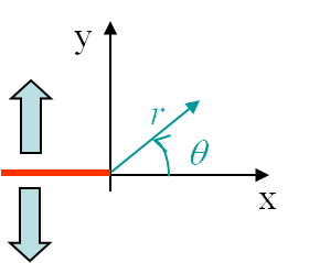
The boundary conditions associated to the first mode, see Picture II.13, were found to be
\begin{equation}\begin{cases} \mathbf{\sigma}_{zz} = 0~~~~\text{or}~~~~ \mathbf{\varepsilon}_{zz} = 0 \\ \mathbf{\sigma}_{yy}(\theta \pm \pi) = 0 \\ \mathbf{\sigma}_{xy}(\theta \pm \pi) = 0 \\ \mathbf{u}_x (\theta) = \mathbf{u}_x (-\theta) \\ \mathbf{u}_y (\theta) = -\mathbf{u}_y (-\theta) \end{cases},\label{eq:bcModeI}\end{equation}
Because of the symmetry with respect to the x-axis of the displacement field $\mathbf{u}$, the expression (\ref{eq:uComponentSeries}) implies $C_2 = C_4 = 0$. As a direct consequence, the unknown functions (\ref{eq:OmegaSeries}) and their derivatives become
\begin{equation}\begin{cases}
\Omega\left(\zeta\right) = &\sum_{\lambda} C_1\zeta^{\lambda+1}=
\sum_{\lambda} C_1r^{\lambda+1}\exp{\left(i\theta\left(\lambda+1\right)\right)}\\ \Omega'\left(\zeta\right) = &\sum_{\lambda} C_1\left(\lambda+1\right)\zeta^{\lambda}=
\sum_{\lambda} C_1\left(\lambda+1\right) r^{\lambda}\exp{\left(i\theta\lambda\right)}\\ \Omega''\left(\zeta\right) = &\sum_{\lambda} C_1\left(\lambda+1\right)\lambda \zeta^{\lambda-1}=
\sum_{\lambda} C_1\left(\lambda+1\right)\lambda r^{\lambda-1}\exp{\left(i\theta\left(\lambda-1\right)\right)}\\ \omega'\left(\zeta\right) = &\sum_{\lambda} C_3\zeta^{\lambda+1}=
\sum_{\lambda} C_3r^{\lambda+1}\exp{\left(i\theta\left(\lambda+1\right)\right)}\\ \omega''\left(\zeta\right) = &\sum_{\lambda} C_3\left(\lambda+1\right)\zeta^{\lambda}=
\sum_{\lambda} C_3\left(\lambda+1\right) r^{\lambda}\exp{\left(i\theta\lambda\right)}
\end{cases},\label{eq:OmegaSeriesModeI}\end{equation}
which allows writing the stress components (\ref{eq:stressAiry}) as
\begin{equation}\begin{cases} \mathbf{\sigma}_{xx} = & \Omega' +\bar{\Omega}' -\frac{\bar{\zeta}\Omega''+\zeta\bar{\Omega}'' + \omega'' + \bar{\omega}''}{2}= \sum_{\lambda}\left(\lambda+1\right) r^\lambda
\left[\left(2C_1-C_3\right)\cos{\left(\lambda\theta\right)} - C_1\lambda \cos{\left(\left(\lambda-2\right)\theta\right)}\right]\\\mathbf{\sigma}_{yy} = &\Omega' +\bar{\Omega}' +\frac{\bar{\zeta}\Omega''+\zeta\bar{\Omega}'' + \omega'' + \bar{\omega}''}{2}=\sum_{\lambda}\left(\lambda+1\right) r^\lambda \left[\left(2C_1+C_3\right)\cos{\left(\lambda\theta\right)} + C_1\lambda \cos{\left(\left(\lambda-2\right)\theta\right)}\right] \\
\mathbf{\sigma}_{xy} = & i \frac{\zeta\bar{\Omega}''-\bar{\zeta}\Omega'' + \bar{\omega}''- \omega'' }{2}= \sum_{\lambda}\left(\lambda+1\right) r^\lambda \left[ C_1\lambda \sin{\left(\left(\lambda-2\right)\theta\right)}+C_3 \sin{\left(\lambda\theta\right)} \right]\end{cases} \label{eq:stressAiryModeI}, \end{equation}
where we have used the identity $\cos{\left(\left(\lambda\pm 2\right)\theta\right)}=\cos{\lambda\theta}\cos{2\theta}\mp \sin{\lambda\theta}\sin{2\theta}$.
As the crack is stress-free (\ref{eq:bcModeI}), $\mathbf{\sigma}_{yy}\left(\theta=\pm\pi\right)=\mathbf{\sigma}_{xy}\left(\theta=\pm\pi\right)=0$ and the last two equations of (\ref{eq:stressAiryModeI}) leads to the system
\begin{equation} \left(\begin{array}{cc} \left(2+\lambda\right)\cos{\lambda\pi} & \cos{\lambda \pi}\\ \lambda\sin{\lambda\pi} & \sin{\lambda \pi} \end{array}\right) \left( \begin{array}{c} C_1\\ C_3 \end{array} \right) =\left( \begin{array}{c} 0\\ 0 \end{array} \right),
\end{equation}
which, in order to admit non-trivial solutions, implies the relation
\begin{equation} 0=\left|\begin{array}{cc} \left(2+\lambda\right)\cos{\lambda\pi} & \cos{\lambda \pi}\\ \lambda\sin{\lambda\pi} & \sin{\lambda \pi} \end{array}\right|=\sin{2\lambda\pi}. \end{equation}
This last equation is satisfied for $\lambda = \frac{n}{2}$, with $n$ = -1, 0, 1, ... as $\lambda > -1$ for the displacement field to remain finite. Since the displacement field is in $r^{\lambda+1}$ and the stress field in $r^\lambda$, the dominant term near the crack tip is obtained for $\lambda = -\frac{1}{2}$. So when considering the asymptotic solution we only retain this dominant term and the terms of higher order ($\lambda = 0, \frac{1}{2}$, ...) are neglected. Finally, as the crack is stress free $\mathbf{\sigma}_{xy}\left(\theta=\pm\pi\right)=0$, and (\ref{eq:stressAiryModeI}) leads to $C_1 = 2C_3$.
Stress field
As the constants and the manifold of $\lambda$ have been determined, we can rewrite the stress field (\ref{eq:stressAiryModeI}) as
\begin{equation}\begin{cases} \mathbf{\sigma}_{xx} = &\frac{1}{4\sqrt{r}} C_1 \left[4\cos{\frac{\theta}{2}}-\cos{\frac{\theta}{2}} +
\cos{\left(\frac{5\theta}{2}\right)}\right] +\mathcal{O}\left(r^0\right)=\frac{1}{\sqrt{r}} C_1 \cos{\frac{\theta}{2}}\left[1-\sin{\frac{\theta}{2}}\sin{\frac{3\theta}{2}}\right]+\mathcal{O}\left(r^0\right) \\ \mathbf{\sigma}_{yy} = & \frac{1}{4\sqrt{r}} C_1 \left[4\cos{\frac{\theta}{2}}+\cos{\frac{\theta}{2}} - \cos{\left(\frac{5\theta}{2}\right)}\right]+\mathcal{O}\left(r^0\right)=\frac{1}{\sqrt{r}} C_1 \cos{\frac{\theta}{2}}\left[1+\sin{\frac{\theta}{2}}\sin{\frac{3\theta}{2}}\right]+\mathcal{O}\left(r^0\right)\\ \mathbf{\sigma}_{xy} = &\frac{1}{4\sqrt{r}}C_1 \left[ \sin{\frac{5\theta}{2}} -\sin{\frac{\theta}{2}} \right]+\mathcal{O}\left(r^0\right) =\frac{1}{\sqrt{r}} C_1 \cos{\frac{\theta}{2}}\sin{\frac{\theta}{2}}\cos{\frac{3\theta}{2}}+\mathcal{O}\left(r^0\right) \end{cases} \label{eq:stressAsympModeItmp}, \end{equation}
where we have used the identities $\cos{a}-\cos{b}=-2\sin{\frac{a-b}{2}}\sin{\frac{a+b}{2}}$ and $\sin{a}-\sin{b}=2\sin{\frac{a-b}{2}}\cos{\frac{a+b}{2}}$. As the stress field tends to infinity at the crack tip, the Stress Intensity Factor (SIF) of the first loading mode has been defined from the more severe stress field $\mathbf{\sigma}_{yy}$ for the crack as
\begin{equation} K_I = \lim_{r\rightarrow 0} \left(\sqrt{2\pi r}\left.\mathbf{\sigma}_{yy}^{\text{mode I}}\right|_{\theta=0} \right) = C_1 \sqrt{2\pi},\label{eq:SIFI}\end{equation}
which allows rewriting the asymptotic stress field (\ref{eq:stressAsympModeItmp}) as
\begin{equation}\begin{cases} \mathbf{\sigma}_{xx} = &\frac{K_I}{\sqrt{2\pi r}} \cos{\frac{\theta}{2}}\left[1-\sin{\frac{\theta}{2}}\sin{\frac{3\theta}{2}}\right]+\mathcal{O}\left(r^0\right) \\ \mathbf{\sigma}_{yy} = &\frac{K_I}{\sqrt{2\pi r}} \cos{\frac{\theta}{2}}\left[1+\sin{\frac{\theta}{2}}\sin{\frac{3\theta}{2}}\right]+\mathcal{O}\left(r^0\right)\\ \mathbf{\sigma}_{xy} = &\frac{K_I}{\sqrt{2\pi r}} \cos{\frac{\theta}{2}}\sin{\frac{\theta}{2}}\cos{\frac{3\theta}{2}}+\mathcal{O}\left(r^0\right) \end{cases} \label{eq:stressAsympModeI}. \end{equation}
The last unknown in this solution is the value of $K_I$. This value actually depends on both the geometry and loading conditions of the sample and its evaluation is the subject of another lecture. Note however its unit: $\text{MPa}\cdot\sqrt{\text{m}}$.
Displacement field
Introducing the constants and the manifold of $\lambda$ in the displacement field (\ref{eq:uComponentSeries}) leads to
\begin{equation}\begin{cases} \mathbf{u}_x&=& \frac{1+\nu}{E}\sqrt{r} C_1\cos{\frac{ \theta}{2}} \left[\kappa-1+2 \sin^2{\frac{\theta}{2}}\right] +\mathcal{O}\left(r\right)\\ \mathbf{u}_y&=& \frac{1+\nu}{E}\sqrt{r} C_1\sin{\frac{ \theta}{2}} \left[\kappa+1-2 \cos^2{\frac{\theta}{2}}\right]+\mathcal{O}\left(r\right)\end{cases},\label{eq:uModeItmp} \end{equation}
which becomes with the definition of $K_I$ (\ref{eq:SIFI})
\begin{equation}\begin{cases} \mathbf{u}_x&=& K_I \frac{1+\nu}{E}\sqrt{\frac{r}{2\pi}} \cos{\frac{ \theta}{2}} \left[\kappa-1+2 \sin^2{\frac{\theta}{2}}\right] +\mathcal{O}\left(r\right)\\ \mathbf{u}_y&=& K_I \frac{1+\nu}{E}\sqrt{\frac{r}{2\pi}}\sin{\frac{ \theta}{2}} \left[\kappa+1-2 \cos^2{\frac{\theta}{2}}\right]+\mathcal{O}\left(r\right)\end{cases},\label{eq:uModeI} \end{equation}
Visualization of the fields
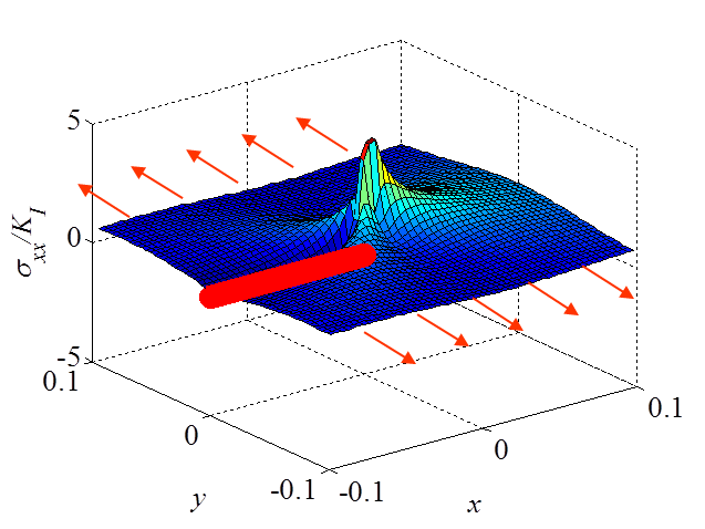
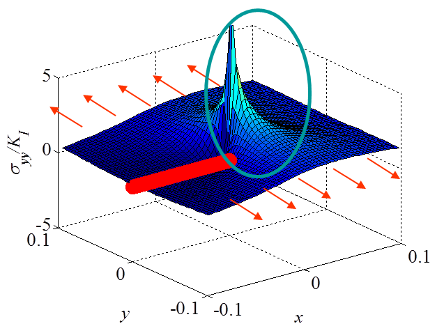
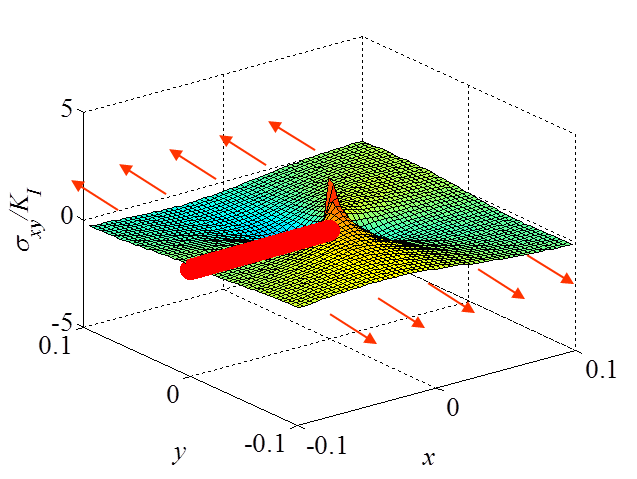
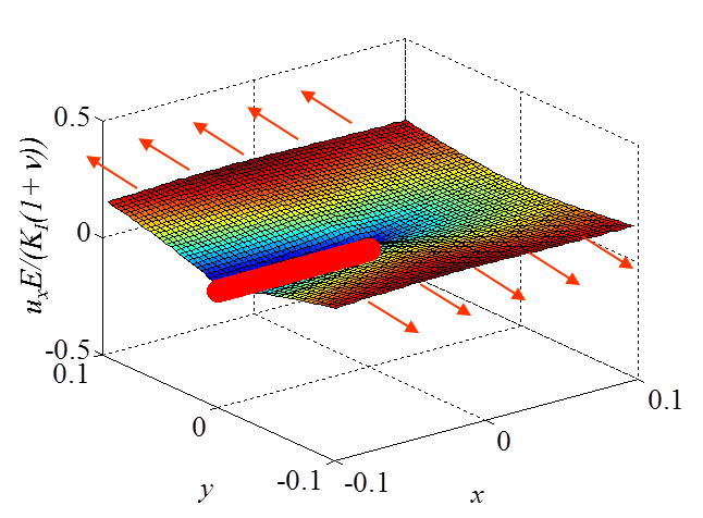
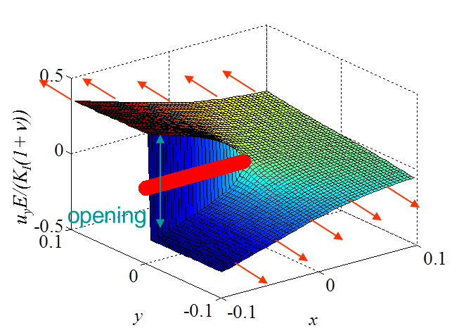
The asymptotic stress field (\ref{eq:stressAsympModeI}) obtained for a Mode I loading is illustrated in Pictures II.14, II.15, and II.16. In particular Picture II.15 represents the "yy"-stress component on which the stress concentration profile, which tends to infinity, is surrounded. The displacement field (\ref{eq:uModeI}) is illustrated in Pictures II.17 and II.18. Of importance is the crack opening profile that can be observed in Picture II.18.
Validity of the solution
It is important to remember that this solution is valid only in a restricted region as it is asymptotic.
Let us first assume there are no plastic deformations. The LEFM asymptotic method thus predicts a stress field in $\frac{1}{\sqrt{r}}$ tending to infinity at the crack tip, see Picture II.19. This is of course unphysical and some irreversible behaviors occur near the crack tip (dark green zone on Picture II.19). The asymptotic solution is thus not valid in this zone. Now faraway of the crack tip, the asymptotic solution has neglected the terms in $r^0$, $\sqrt{r}$, $r$ ... and does not capture the structural response (faraway from the crack tip the asymptotic solution predicts a stress tending to zero, which is not usually the correct answer), see Picture II.19. As a summary, the LEFM solution is not valid faraway from the crack tip and is not valid close to the crack tip in a zone whose size depends on the degree of plastic deformations involved.
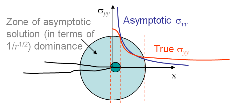
- For some materials, considered as brittle, if the sample is large enough the dark green zone of Picture II.19 remains small enough and there exists a cylindrical zone (light green in Picture II.19), in which the asymptotic solution if valid. In this case the LEFM approach can be used.
- If the material is more ductile, or if the sample is too small, the dark green region becomes bigger with respect to the structural response stress field zone and the region of validity of the asymptotic solution vanishes. LEFM approach cannot be used anymore.
Mode II asymptotic solution
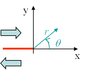
The boundary conditions associated to the second loading mode, see Picture II.13, were found to be
\begin{equation}\begin{cases} \mathbf{\sigma}_{zz} = 0~~~~\text{or}~~~~ \mathbf{\varepsilon}_{zz} = 0 \\ \mathbf{\sigma}_{yy}(\theta \pm \pi) = 0 \\ \mathbf{\sigma}_{xy}(\theta \pm \pi) = 0 \\ \mathbf{u}_x (\theta) = -\mathbf{u}_x (-\theta) \\ \mathbf{u}_y (\theta) = \mathbf{u}_y (-\theta) \end{cases},\label{eq:bcModeII}\end{equation}
Because of the anti-symmetry with respect to the x-axis of the displacement field $\mathbf{u}_x$, the expression (\ref{eq:uComponentSeries}) implies $C_1 = C_3 = 0$. The solution can then be derived as for the Mode I loading.
Stress field
The Stress Intensity Factor (SIF) of the second loading mode has been defined from the more severe stress field $\mathbf{\sigma}_{xy}$ for the crack as
\begin{equation} K_{II} = \lim_{r\rightarrow 0} \left(\sqrt{2\pi r}\left.\mathbf{\sigma}_{xy}^{\text{mode II}}\right|_{\theta=0} \right) ,\label{eq:SIFII}\end{equation}
which allows rewriting the asymptotic stress field as
\begin{equation}\begin{cases} \mathbf{\sigma}_{xx} = & - \frac{K_{II}}{\sqrt{2\pi r}} \sin{\frac{\theta}{2}} \left[2 +\cos{\frac{\theta}{2}}\cos{\frac{3\theta}{2}}\right] +\mathcal{O}\left(r^0\right)\\ \mathbf{\sigma}_{yy} = & \frac{K_{II}}{\sqrt{2\pi r}} \sin{\frac{\theta}{2}} \cos{\frac{\theta}{2}}\cos{\frac{3\theta}{2}}+\mathcal{O}\left(r^0\right) \\ \mathbf{\sigma}_{xy} = &\frac{K_{II}}{\sqrt{2\pi r}} \cos{\frac{\theta}{2}}\left[1-\sin{\frac{\theta}{2}}\sin{\frac{3\theta}{2}}\right]+\mathcal{O}\left(r^0\right)\end{cases} \label{eq:stressAsympModeII} . \end{equation}
The last unknown in this solution is the value of $K_{II}$, which also depends on both the geometry and loading conditions of the sample and its evaluation is the subject of another lecture. Note however its unit: $\text{MPa}\cdot\sqrt{\text{m}}$.
Displacement field
The displacement field reads
\begin{equation}\begin{cases} \mathbf{u}_x&=& K_{II}\frac{1+\nu}{E}\sqrt{\frac{r}{2\pi}} \sin{\frac{ \theta}{2}} \left[\kappa+1+2 \cos^2{\frac{\theta}{2}}\right] +\mathcal{O}\left(r\right)\\ \mathbf{u}_y&=&K_{II}\frac{1+\nu}{E}\sqrt{\frac{r}{2\pi}} \cos{\frac{ \theta}{2}} \left[1-\kappa+2 \sin^2{\frac{\theta}{2}}\right] +\mathcal{O}\left(r\right)\end{cases},\label{eq:uModeII} \end{equation}
Visualization of the fields
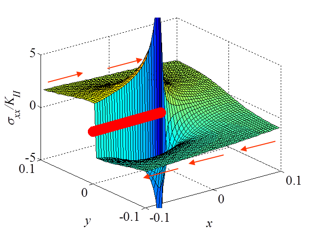
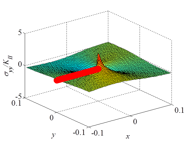
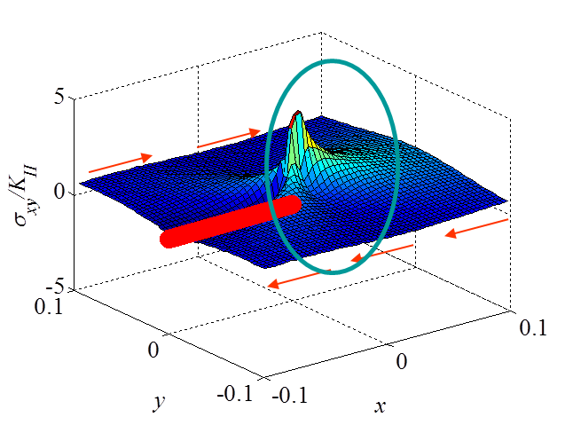
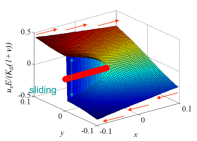
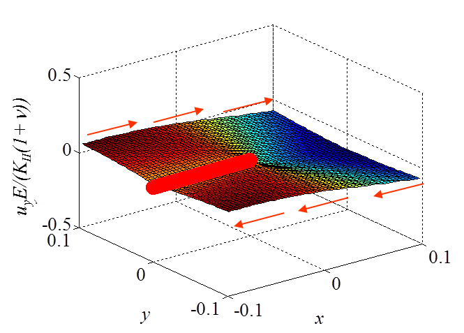
The asymptotic stress field (\ref{eq:stressAsympModeII}) obtained for a Mode II loading is illustrated in Pictures II.21, II.22, and II.23. This last Picture II.23 represents the "xy"-stress component on which the stress concentration profile, which tends to infinity, is surrounded. The displacement field (\ref{eq:uModeII}) is illustrated in Pictures II.24 and II.25. The crack sliding profile can be observed in Picture II.24.
Only one mode, the Mode III or shearing mode, remains to be studied. However as this mode involves an out-of-plane shearing, the resolution method is slightly different as it is shown in the next section.